IF Function in Excel (7 Easy Examples)

If you want Excel to return one value when a condition is true and a different value when it is false, the IF function is what you are looking for.

It is one of the most popular functions in Excel, and once you have it down, you will reach for it in almost every workbook you build.

In Excel 365, you can also feed IF a range and the results spill into the cells below.

In this article, I will show you how to use the IF function with seven practical examples, including the basic syntax, AND/OR conditions, nested IFs, and the spilling form.

Table of Contents

IF Function Syntax in Excel

The IF function takes a logical test and returns one value if the test is true, and another value if it is false.

=IF(logical_test, value_if_true, [value_if_false])

logical_test: the condition to evaluate (for example B2>=60 or A2="Yes").
value_if_true: what to return when the test is true.
value_if_false: what to return when the test is false. This argument is optional. If you skip it, IF returns the word FALSE, which is rarely useful.

When to Use IF Function

IF shows up any time you need a quick branching decision in a cell. Common use cases:

Pass or Fail style labels based on a threshold
Comparing two cells and labeling the result (over or under, higher or lower)
Running a calculation only when a condition is met (a bonus when sales hit target, for example)
Checking whether a cell is blank or filled in
Combining with AND or OR to test multiple conditions in one formula
Nesting for tiered logic like letter grades or commission tiers

Example 1: Pass or Fail Based on a Score

Let’s start with a simple example.

Below is the dataset with student names in column A and their final scores in column B. Column C is where the result will go.

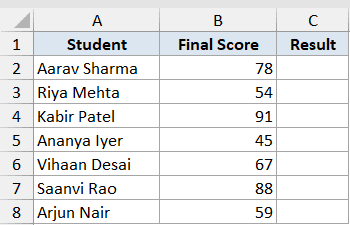
Excel table with columns for Student, Final Score, and empty Result cells for seven students with scores from 45 to 91

The passing score is 60, so anyone scoring 60 or above passes and everyone else fails.

Here is the formula:

=IF(B2>=60, "Pass", "Fail")

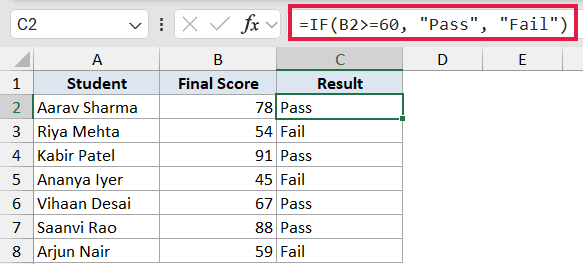
This formula checks whether the value in cell B2 is 60 or higher. If it is, the function returns “Pass”. If the score is below 60, it returns “Fail”.

Copy the formula down to the rest of the rows, and each student gets their own result based on their score.

Note: text values need to be wrapped in double quotes. Without them, Excel returns a #NAME? error because it tries to read Pass and Fail as named ranges.

Example 2: Over or Under Target

Here is another practical scenario.

Below is the dataset showing each sales rep, their quarterly target in column B, and their actual sales in column C. Column D is where we want the status.

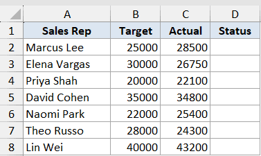
Excel IF function dataset with columns for Sales Rep, Target, Actual, and an empty Status column for calculations

We want one formula that fills the entire Status column at once, showing “Over Target” when actual sales beat the target and “Under Target” otherwise.

Here is the formula:

=IF(C2:C8>B2:B8, "Over Target", "Under Target")

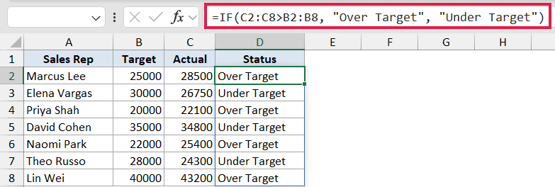
Excel formula bar showing an IF function spilling results into column D to compare actual sales against targets

Because the formula passes two ranges (C2:C8 and B2:B8) instead of single cells, Excel 365 spills the result across D2:D8. You only need to enter the formula once in cell D2, and the entire column fills in automatically.

This is the dynamic array form of IF. When you click any cell inside the spilled range, you will see a thin blue border around it.

Note: if any cell inside D2:D8 already has something in it, the spill will fail with a #SPILL! error. Clear the cells first and the formula will work.

Example 3: Multiple Conditions With AND

Let’s step it up.

Below is the dataset with each student’s Math score in column B and English score in column C. We want to mark a student as Pass only when both scores are 60 or higher.

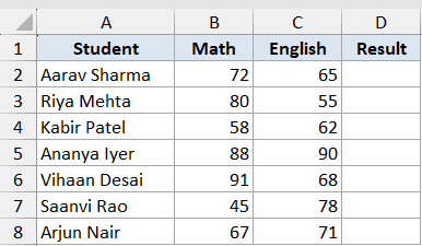
Excel dataset with columns for Student name, Math score, English score, and an empty Result column for IF function testing

A single comparison like in Example 1 will not work here, because we need two conditions to be true at the same time. We wrap the IF inside an AND.

Here is the formula:

=IF(AND(B2>=60, C2>=60), "Pass", "Fail")

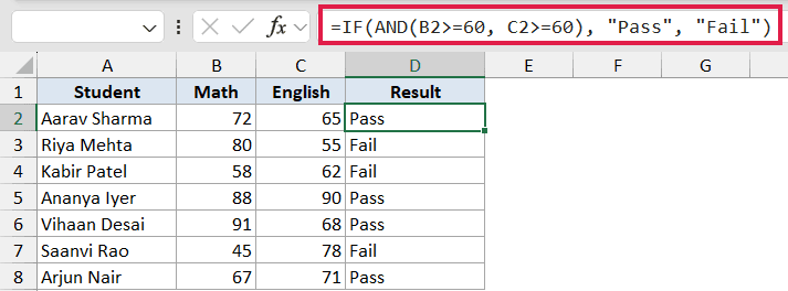
Excel IF formula with AND function in the formula bar, evaluating student Math and English scores for Pass or Fail results

The AND function returns TRUE only when both of its arguments are TRUE. If either Math or English drops below 60, AND returns FALSE, and the IF returns “Fail”.

Looking at the result, Riya scored 80 in Math but 55 in English, so she fails. Aarav has 72 and 65, so he passes both subjects.

Pro Tip: AND collapses a range of comparisons into a single TRUE or FALSE value, so this formula runs row by row rather than spilling. To get the same check to spill across all rows in Excel 365, multiply the conditions instead: =IF((B2:B8>=60)*(C2:C8>=60), "Pass", "Fail"). Multiplying TRUE/FALSE arrays gives 1 only when both are TRUE, and IF treats any non-zero number as TRUE.

Example 4: Multiple Conditions With OR

Let’s look at a different logic case.

Below is a customer list showing whether each customer is a member in column B and the value of their current order in column C. We want to flag who qualifies for a discount.

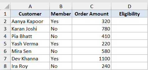
If Function Dataset Example 4 showing customer names, membership status, and order amounts in an Excel table

A customer qualifies for a discount when they are a member OR when their order is over 500. Either condition on its own is enough.

Here is the formula:

=IF(OR(B2="Yes", C2>500), "Discount", "No Discount")

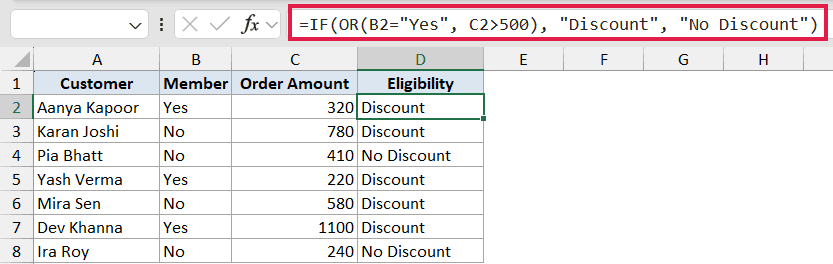
Excel IF formula using OR logic to determine discount eligibility based on member status or order amount over 500

OR returns TRUE if even one of the conditions is TRUE. So Aanya gets a discount because she is a member even though her order is small, and Karan gets one because his order is 780 even though he is not a member.

Pia and Ira fail both checks (no membership and order under 500), so they land on “No Discount”. Yash still qualifies on membership alone, even though his order is only 220.

If you replaced OR with AND in the same formula, only customers who are both members AND placing an order over 500 would get a discount. OR is the more generous of the two.

Example 5: Nested IF for Letter Grades

Here is a more complex use case.

Below is a list of students and their final scores. We want to convert each score into a letter grade: 90 and above is an A, 80s a B, 70s a C, 60s a D, and anything below 60 is an F.

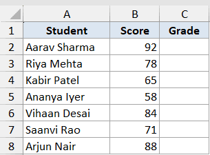
Excel IF function dataset showing a table with Student names in column A and numerical Scores in column B

A single IF only handles two outcomes (true or false), so for five grade bands, we nest one IF inside another.

Here is the formula:

=IF(B2>=90, "A", IF(B2>=80, "B", IF(B2>=70, "C", IF(B2>=60, "D", "F"))))

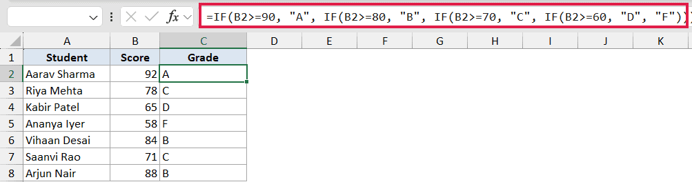
Excel formula bar showing a nested IF function for grading scores, with student names and letter grades in a table

How this formula works:

The first IF checks if the score is 90 or higher. If yes, it returns “A”.
If not, the second IF takes over as the value_if_false of the first IF, and it checks if the score is 80 or higher. If yes, return “B”.
The same pattern continues down through C, D, and finally F as the fallback when nothing else matched.

Reading nested IFs is easier when you think of them as a sequence of “if not this, then check the next thing”.

Pro Tip: In Excel 2019 and later, you can also write the same logic using the IFS function: =IFS(B2>=90, "A", B2>=80, "B", B2>=70, "C", B2>=60, "D", TRUE, "F"). IFS is shorter and easier to read because you do not need to close four sets of parentheses at the end. The nested IF still works in older versions of Excel where IFS does not exist, so it is worth knowing both.

Example 6: IF With a Conditional Calculation

Now let’s use IF to return a calculation instead of a text label.

Below is a list of sales reps and their sales for the quarter. We want to pay out a 10% bonus, but only to reps who hit at least 10,000 in sales.

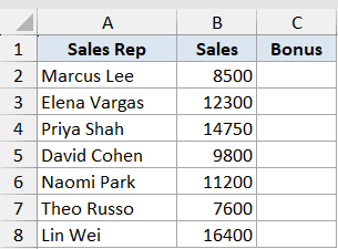
Excel IF function dataset example 6 showing a table with Sales Rep names and Sales figures with an empty Bonus column

Anyone below 10,000 gets a bonus of 0. Anyone at or above 10,000 gets 10% of their sales.

Here is the formula:

=IF(B2>=10000, B2*0.1, 0)

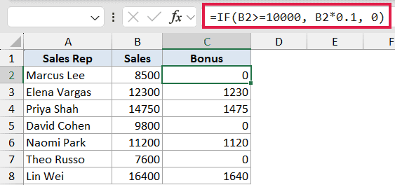
Excel formula bar showing IF function calculating a 10 percent bonus for sales over 10000 in a sales data table

When the condition is true, the formula multiplies B2 by 0.1 (which is 10%). When it is false, the formula returns 0. The result is a real number, not a text label, which means you can sum the bonus column, average it, or feed it into further calculations.

This pattern is one of the most common real-world uses of IF. You set a threshold, and the formula either runs a calculation or returns a fallback value depending on whether the threshold is met.

Example 7: Blank vs Complete

Let’s wrap up with another spilling example.

Below is a task list. Some tasks have a completion date in column B, and others are still blank because the work has not been finished yet.

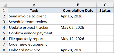
Excel IF Function Dataset Example 7 showing a task list with completion dates and an empty status column

We want column C to show “Pending” for blank rows and “Complete” for filled rows, all from a single formula.

Here is the formula:

=IF(B2:B8="", "Pending", "Complete")

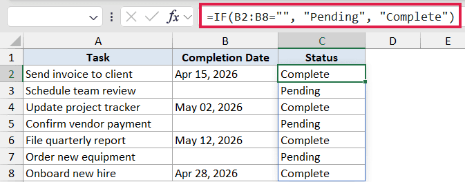
Excel formula bar showing a spilled IF function evaluating a range to return Pending or Complete status for tasks

The condition B2:B8="" returns an array of TRUE and FALSE values, one for each row. IF then turns each TRUE into “Pending” and each FALSE into “Complete”, and the entire status column fills in from a single formula entered into C2.

This is the same dynamic array behavior we saw in Example 2. The difference is the test itself: instead of comparing two ranges, we are checking each cell for blank.

Note: this checks for cells that are truly empty or contain an empty string. If a cell has a single space in it, Excel still sees that as text and the formula will treat it as Complete. To also catch space-only cells, use =IF(TRIM(B2:B8)="", "Pending", "Complete").

Tips & Common Mistakes

Wrap text values in double quotes. IF(B2="Yes", ...) works. IF(B2=Yes, ...) throws a #NAME? error because Excel reads Yes as a named range. The same applies to the return values.
The third argument is optional, but worth using. If you skip value_if_false, IF returns the word FALSE whenever the condition is not met. That is almost never what you want. Pass something explicit, even if it is just "" for a blank cell.
Watch the closing parentheses. Nested IFs can need three, four, or five closing brackets at the end. If you get a “There’s a problem with this formula” error, count the opening and closing parentheses. Excel highlights matching pairs as you type, which helps.
AND and OR collapse ranges to a single value. As shown in Example 3, putting AND(B2:B8>=60, C2:C8>=60) inside an IF does not spill row by row. Use (B2:B8>=60)*(C2:C8>=60) for the spilling version, or use a per-row formula filled down.
For more than three or four tiers, consider IFS or SWITCH. Nested IF gets hard to read past four levels. IFS (Excel 2019+) handles the same logic with cleaner syntax, as shown in the Pro Tip in Example 5. SWITCH works well when you are matching exact values rather than ranges.
IF is not case-sensitive by default. IF(A2="YES", ...) and IF(A2="yes", ...) return the same result. If you need a case-sensitive match, wrap the test in EXACT, like =IF(EXACT(A2, "Yes"), "Member", "Non-Member").

IF is where most people start with logical formulas in Excel. Once you have the basic syntax down, the AND, OR, nested, and spilling forms all build on the same idea: test a condition and return one of two values.

The seven examples above cover the patterns I reach for most often in real work. Try a few of them on your own data and you will see why IF shows up in nearly every workbook.

List of All Excel Functions

Related Excel Functions / Articles: