SWITCH Function in Excel

If you need one formula to turn codes or categories into clear results, the SWITCH function can save you from writing a long chain of IF formulas.

It checks one expression against a list of values and returns the result tied to the first match. In Excel 365, you can also feed SWITCH a range and the results spill into the cells below.

In this article, I’ll show you six practical ways to use SWITCH, including defaults, conditions, calculations, and weekday schedules.

SWITCH Function Syntax in Excel

The SWITCH function uses the following syntax:

=SWITCH(expression, value1, result1, [default or value2, result2],…[default or value3, result3])

• expression is the value or calculation Excel checks.
• value1 is the first value compared with the expression.
• result1 is returned when value1 matches the expression.
• value2, result2 and later pairs are optional. You can supply up to 126 value and result pairs.
• default is optional and must be the final argument. Excel returns it when no value matches.

When to Use SWITCH Function

• Convert short, fixed code lists into readable labels.
• Return a different calculation for each category.
• Group numeric values into bands with SWITCH(TRUE,...).
• Map weekday numbers or other repeated values to a schedule.

Example 1: Map Numeric Codes to Actions

Let’s start with a short list of inspection codes.

Below is the dataset with rental IDs and the code recorded after each inspection.

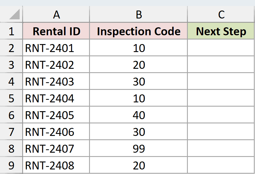
I want Excel to return the correct next step for each code and flag any code outside the approved list.

Here is the formula:

=SWITCH(B2:B9,10,"Return to Stock",20,"Clean",30,"Repair",40,"Supervisor Review","Unknown Code")

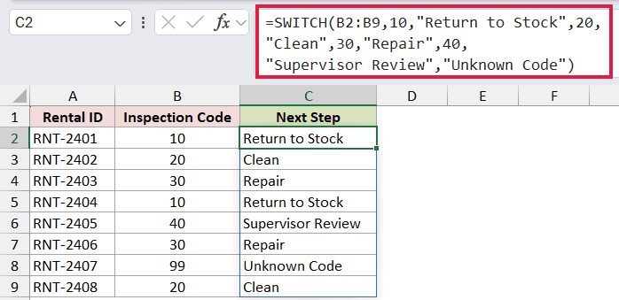
SWITCH compares every value in B2:B9 with 10, 20, 30, and 40. It returns the paired instruction when it finds a match.

The final text, "Unknown Code", is the default. That is why code 99 returns a useful warning instead of an error.

In Excel 365, the XLOOKUP function is easier to maintain when these mappings live in a worksheet table and change often. SWITCH works well when the list is short and fixed inside the formula.

Example 2: Classify Text Codes by Prefix

SWITCH can also evaluate the result of another function.

Below is the dataset with pallet IDs and storage codes whose first letter identifies the handling zone.

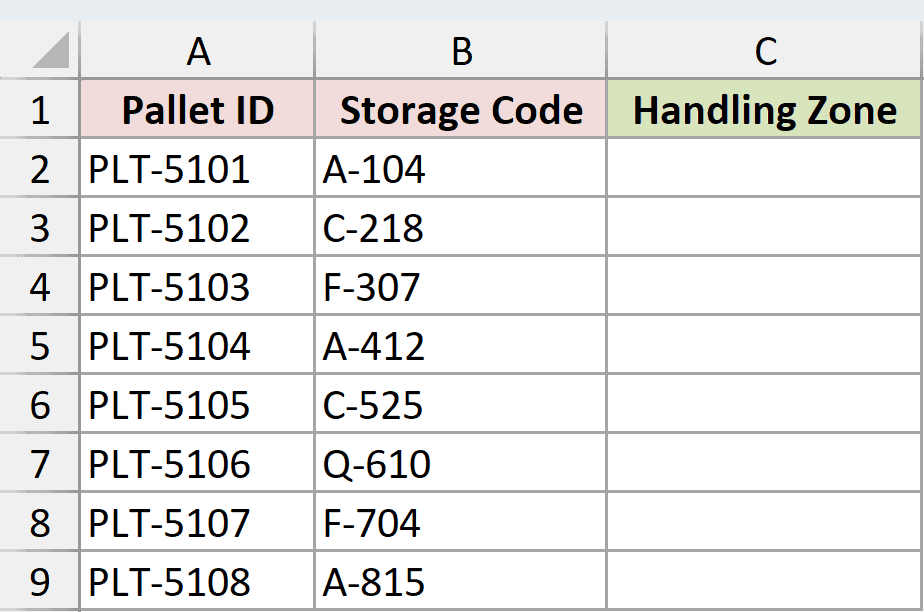
I want to extract each first letter and translate it into Ambient, Chilled, or Frozen.

Here is the formula:

=SWITCH(LEFT(B2:B9,1),"A","Ambient","C","Chilled","F","Frozen","Check Code")

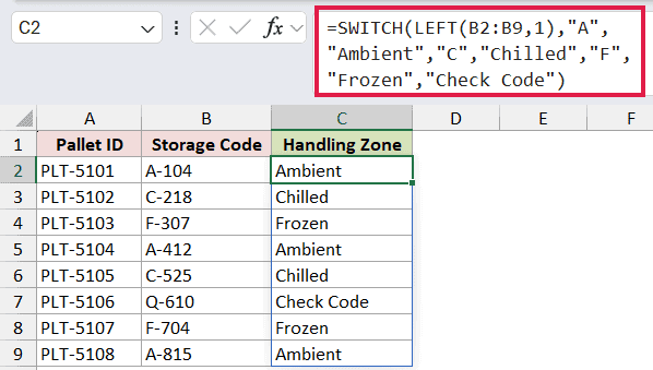
The LEFT function returns the first character from every storage code. SWITCH then compares those letters with "A", "C", and "F".

The Q-610 code does not match any listed letter, so the default result is "Check Code".

Example 3: Use a Default Result

This example shows what happens when a formula does not include a default.

Below is the dataset with payment IDs and method codes. The last two columns compare the two versions of the formula.

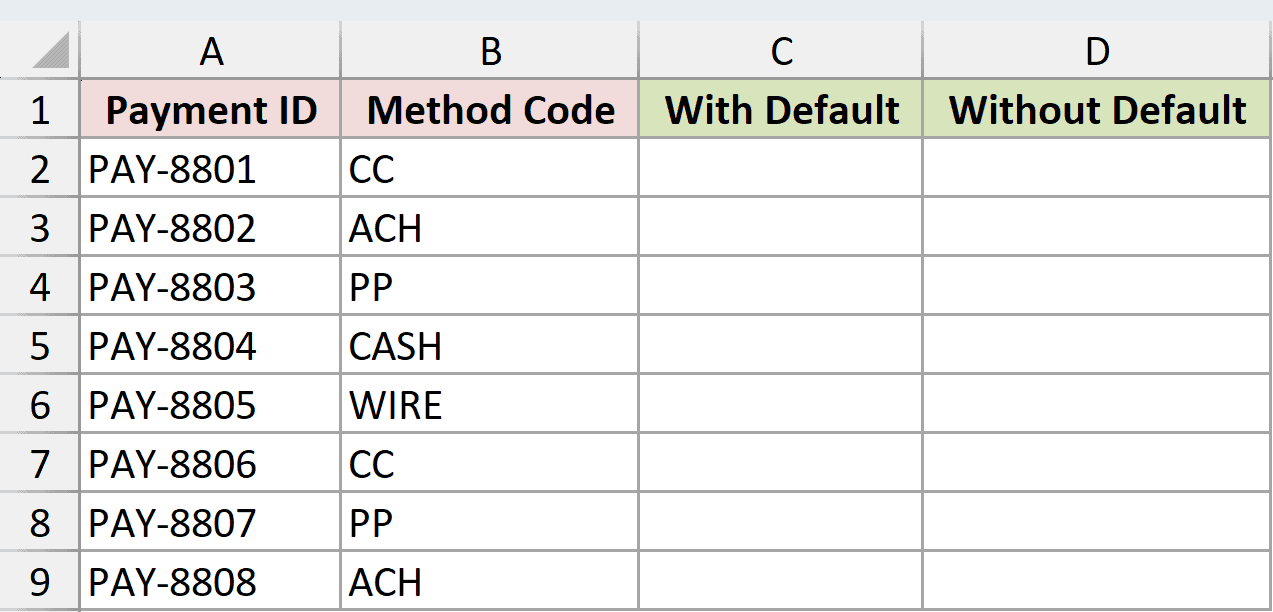
I want the first formula to label unfamiliar codes for review instead of returning an error.

Here is the formula with a default result:

=SWITCH(B2:B9,"CC","Credit Card","ACH","Bank Transfer","PP","PayPal","CASH","Cash","Review Code")

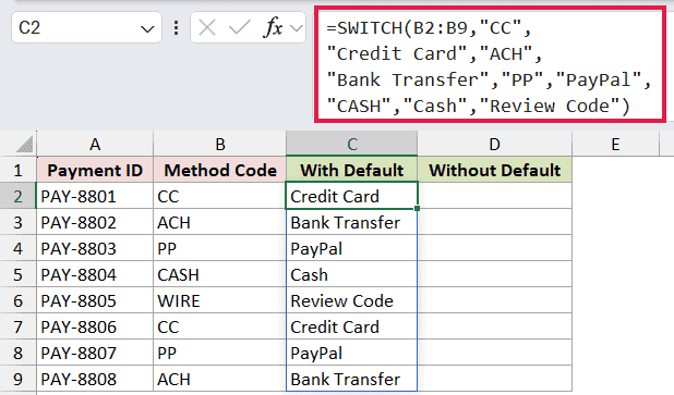
The WIRE entry has no matching value, so the formula returns "Review Code".

Here is the same formula without a default result:

=SWITCH(B2:B9,"CC","Credit Card","ACH","Bank Transfer","PP","PayPal","CASH","Cash")

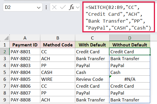
The known codes still return the same labels. The WIRE entry now returns #N/A because SWITCH reaches the end of the formula without finding a match.

Pro Tip: Put the default at the end without a paired result. If you omit it, any unmatched expression returns #N/A.

Example 4: Test Multiple Conditions With SWITCH

SWITCH can also test ordered conditions.

Below is the dataset with request IDs and the number of hours taken to send the first response.

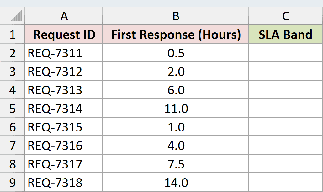
I want to place each request into the first response-time band whose condition is true.

Here is the formula:

=SWITCH(TRUE,B2:B9<=1,"Immediate",B2:B9<=4,"Same Shift",B2:B9<=8,"Monitor","Escalate")

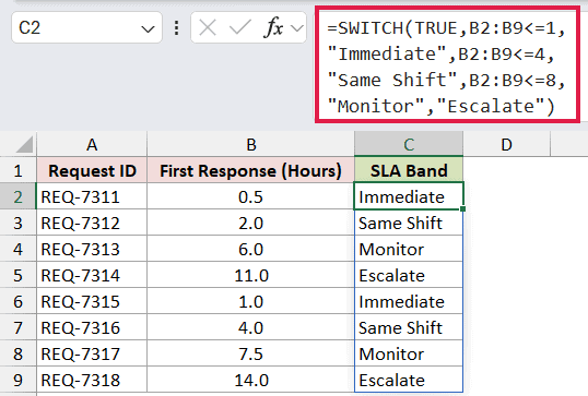
The expression is TRUE, so each condition becomes a possible match. Excel checks the conditions from left to right and returns the result for the first one that evaluates to TRUE.

A response time of 0.5 hours matches the first condition. A response time of 6 hours skips the first two conditions and returns "Monitor".

In Excel 365, the IFS function can handle the same ordered tests with =IFS(B2:B9<=1,"Immediate",B2:B9<=4,"Same Shift",B2:B9<=8,"Monitor",TRUE,"Escalate").

SWITCH remains useful when one formula mixes exact values and condition results.

Pro Tip: Put the narrowest thresholds first. If the condition B2:B9<=8 came first, every value up to 8 would stop there and the smaller bands would never run.

Example 5: Return Different Calculations by Category

The result arguments can contain calculations, not just labels.

Below is the dataset with job IDs, billing models, hours, units, and an empty charge column.

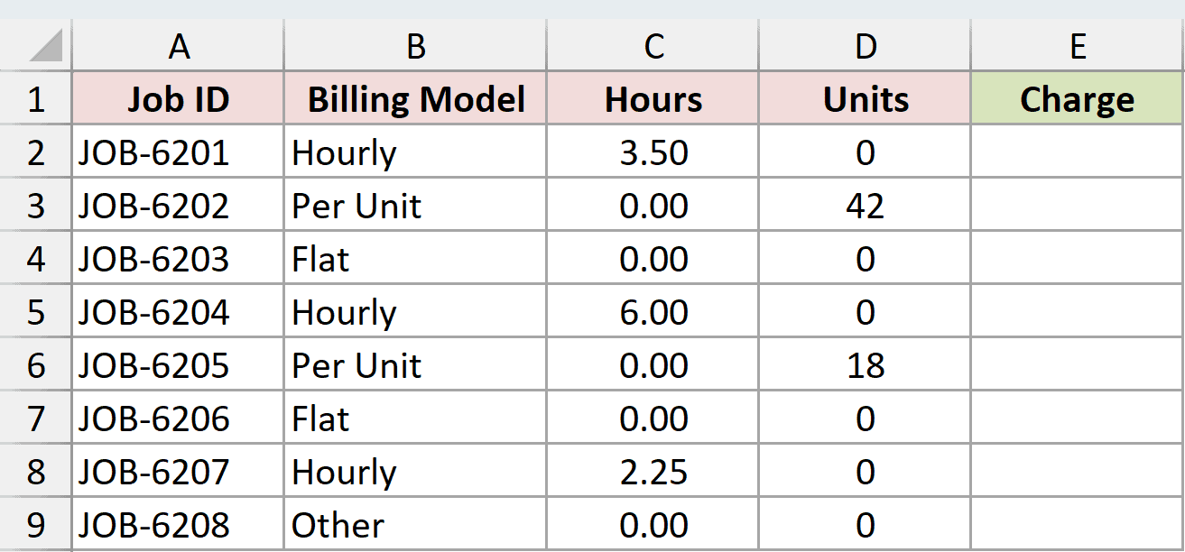
I want one formula to calculate the charge that belongs to each billing model.

Here is the formula:

=SWITCH(B2:B9,"Hourly",C2:C9*95,"Per Unit",D2:D9*12,"Flat",500,0)

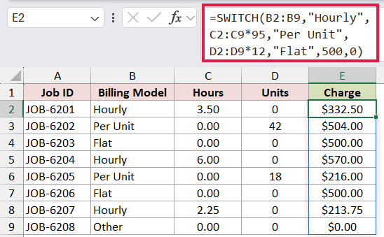
Hourly jobs multiply hours by $95. Per Unit jobs multiply units by $12, while Flat jobs return $500.

The default is 0, so the unsupported "Other" model does not create an error. The spilled results range from $0 to $570 for this dataset.

Example 6: Build a Weekday Schedule

A weekday number can also drive a receiving schedule.

Below is the dataset with eight delivery dates covering Monday, September 7, 2026, through the following Monday.

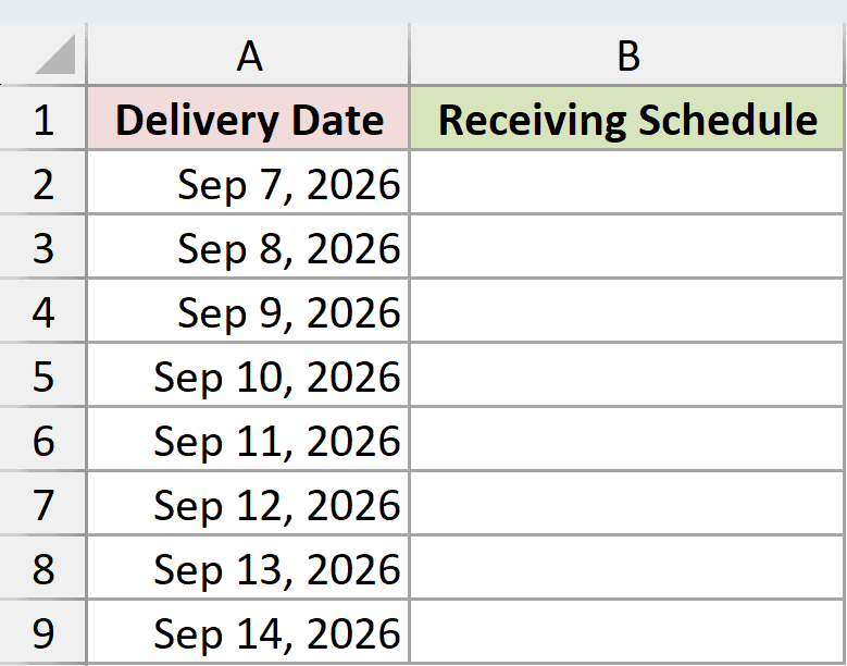
I want to assign each weekday to a dock and mark weekend deliveries as closed.

Here is the formula:

=SWITCH(WEEKDAY(A2:A9,2),1,"Dock A",2,"Dock A",3,"Dock B",4,"Dock B",5,"Dock C","Closed")

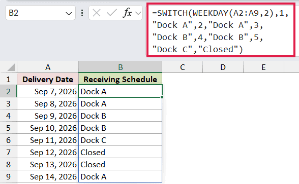
With return type 2, the WEEKDAY function numbers Monday through Sunday as 1 through 7. SWITCH sends Monday and Tuesday to Dock A, Wednesday and Thursday to Dock B, and Friday to Dock C.

Saturday and Sunday have no listed match, so both return the default "Closed". The CHOOSE function is another option when your numeric codes are consecutive, but SWITCH makes the weekend fallback especially clear.

Tips & Common Mistakes

• SWITCH returns the result for the first matching value. If the same value appears twice, later matches are ignored.
• The default argument is optional, but leaving it out causes unmatched values to return #N/A.
• You can use up to 126 value and result pairs because Excel functions accept no more than 254 arguments.
• SWITCH is available in Excel 2019 and later. The spilling formulas shown here require a version of Excel with dynamic arrays, such as Excel 365.
• If Excel applies the implicit-intersection operator, SWITCH returns one row’s result instead of a spill. In Excel 2019, use a row-level formula and copy it down.
• A blocked spill area returns #SPILL!. Clear the cells in the intended output range and let the formula fill them automatically.

I’ve shown you how SWITCH handles fixed mappings, defaults, ordered conditions, calculations, and schedules. I hope you found this article helpful.

List of All Excel Functions

Related Excel Functions / Articles:

• Multiple If Statements in Excel (Nested IFs, AND/OR) with Examples
• XLOOKUP vs VLOOKUP in Excel
• IF Function in Excel
• Using LET in Excel
• MATCH Function in Excel