INDEX Function in Excel (6 Easy Examples)

The INDEX function returns a value from a range based on the row and column position you give it. This article walks through six practical examples, from simple positional lookups to two-way and multi-criteria lookups using INDEX with MATCH. In Excel 365, INDEX can also return an entire row or column as an array that spills into the cells below.

Table of Contents

INDEX Function Syntax in Excel

INDEX has two forms. The most common one is the array form:

=INDEX(array, row_num, [column_num])

array is the range of cells you want to pull a value from.
row_num is the row position within that range. The first row of the range is 1.
column_num is the column position within the range. This is optional when the range is a single column or single row.

There is also a reference form, =INDEX(reference, row_num, [column_num], [area_num]), which lets you point at more than one range and pick a value from a chosen area.

One handy trick works in both forms. Setting row_num=0 returns a whole column, and setting column_num=0 returns a whole row.

When to Use INDEX Function

When you want to grab a value by its position in a list, like the 4th item or the 2nd column.
When you need a more flexible alternative to VLOOKUP by pairing INDEX with MATCH.
When the value you want sits to the left of your lookup column, which VLOOKUP can’t handle.
When you need a two-way lookup that finds a value at the intersection of a row and a column.
When you want to return a whole row or column and feed it into a function like SUM.

Example 1: Pull an Item by Position

Let’s start with the simplest use of INDEX, pulling a value by its row number.

Below is the dataset in A1:B7 with two columns, “Employee” and “Department”. It lists six people and the team each one belongs to.

Excel dataset with employee names and departments, showing a row position input of 4 for an INDEX function example

We want to return the employee who sits in the 4th position of the list, where the position number is in cell D2.

Here is the formula:

=INDEX(A2:A7,D2)

Excel formula bar showing =INDEX(A2:A7,D2) to return the employee name in row 4 of the data range

The row_num argument tells INDEX which item to return. Since D2 holds 4, the formula counts down to the 4th name in A2:A7 and returns Priya Nair. Change D2 to any number from 1 to 6 and the result updates to that position.

Example 2: INDEX + MATCH Lookup

Now let’s pair INDEX with the MATCH function to build a lookup that works like VLOOKUP but with more flexibility.

Below is the dataset in A1:C7 with three columns, “Product ID”, “Product”, and “Price”. Each row holds a product code, its name, and its price. The lookup ID is in E2.

Excel dataset with Product ID, Product, and Price columns, plus a lookup table for ID P-104 to demonstrate INDEX function

We want to find the price for the product with ID P-104.

Here is the formula:

=INDEX(C2:C7,MATCH(E2,A2:A7,0))

Excel formula bar showing INDEX MATCH function to look up price for Product ID P-104 in a table

How this formula works:

MATCH(E2,A2:A7,0) looks for P-104 in the range A2:A7 and returns its position, which is 4. The 0 forces an exact match.
INDEX(C2:C7, 4) then returns the value in the 4th position of the Price column, which is 45.

In Excel 365 and 2021, the XLOOKUP function does the same job more directly with =XLOOKUP(E2,A2:A7,C2:C7). INDEX+MATCH is worth knowing because it works in every version of Excel.

Pro Tip: Unlike VLOOKUP, which relies on a fixed column index number, INDEX+MATCH keeps working when you insert or delete columns between the lookup and return ranges. The references shift along with your data instead of pointing at the wrong column.

Example 3: Left-Side (Reverse) Lookup

Here’s a case where VLOOKUP falls short and INDEX+MATCH shines.

Below is the dataset in A1:C7 with three columns, “Name”, “City”, and “Email”. The names sit in the first column and the emails sit in the last column. The email to look up is in E2.

Excel dataset with columns for Name, City, and Email, plus a lookup table for finding a name by email address

We want to find the name that belongs to a given email, where the answer sits to the left of the lookup column.

Here is the formula:

=INDEX(A2:A7,MATCH(E2,C2:C7,0))

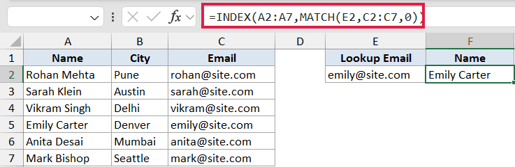
Excel formula bar showing INDEX MATCH lookup function returning Emily Carter based on email address in cell E2

MATCH finds emily@site.com in the Email column (C2:C7) and returns its position, 4. INDEX then returns the value in the 4th position of the Name column (A2:A7), which is Emily Carter.

This is something VLOOKUP can’t do, since it only searches the first column and returns values to the right. INDEX+MATCH points at any two columns you like, so the return range can sit to the left of the lookup range.

Example 4: Two-Way Lookup (Row and Column)

Sometimes you need to find a value at the crossing point of a row and a column. INDEX with two MATCH functions handles this nicely.

Below is the dataset in A1:D6 with four columns, “Region”, “Q1”, “Q2”, and “Q3”. Each row is a region and each column after the first is a quarter, holding revenue figures. The region is picked in F2 and the quarter in G2.

Index Function Dataset Example 4 showing a revenue table with regions and quarters and a lookup table for East Q3

We want the revenue at the intersection of the chosen region and the chosen quarter.

Here is the formula:

=INDEX(B2:D6,MATCH(F2,A2:A6,0),MATCH(G2,B1:D1,0))

Excel formula bar showing INDEX MATCH function for a two-way lookup of East region Q3 revenue in a data table

How this formula works:

MATCH(F2,A2:A6,0) finds the row for the chosen region. East is the 3rd region, so this returns 3.
MATCH(G2,B1:D1,0) finds the column for the chosen quarter. Q3 is the 3rd quarter in the header, so this returns 3.
INDEX(B2:D6, 3, 3) returns the value at the 3rd row and 3rd column of the data, which is 171.

Example 5: Return a Whole Column (Spill)

This is where INDEX shows off its dynamic-array side. Setting one of the position arguments to 0 returns an entire row or column.

Below is the dataset in A1:C7 with three columns, “Salesperson”, “Units”, and “Revenue”. Each row holds a name, the units sold, and the revenue. The spilled output starts in E2, with the header “Revenue (spilled)” in E1.

Index Function Dataset Example 5 showing a sales table with columns for Salesperson, Units, and empty Revenue spilled cells

We want to pull the entire Revenue column out as a single spilling array.

Here is the formula:

=INDEX(B2:C7,0,2)

Excel formula bar showing =INDEX(B2:C7,0,2) returning a spilled array of revenue values in column E

Setting column_num to 2 picks the 2nd column of B2:C7, which is Revenue. Setting row_num to 0 means “all rows of that column.” In Excel 365 the result spills down E2:E7, returning 1200, 1675, 990, 1830, 1440, and 1560.

You can also wrap this in another function. For example, =SUM(INDEX(B2:C7,0,2)) totals a column chosen by its position number, which is handy when the column you want changes.

Pro Tip: The 0 trick is what makes INDEX so flexible. Use row_num=0 to return a whole column and column_num=0 to return a whole row. In Excel 365 the result spills on its own. In older versions you select the output cells first and confirm with Ctrl+Shift+Enter.

Example 6: Multi-Criteria Lookup

When one lookup value isn’t enough to find a unique row, you can match on several criteria at once.

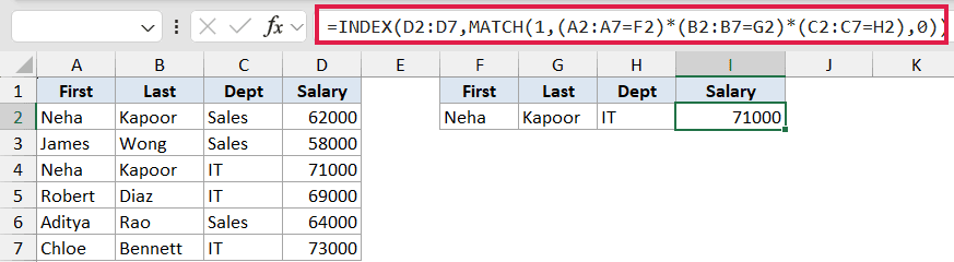
Below is the dataset in A1:D7 with four columns, “First”, “Last”, “Dept”, and “Salary”. Notice there are two rows for Neha Kapoor, one in Sales and one in IT, so a single name lookup wouldn’t be enough. The three criteria are in F2, G2, and H2.

Excel dataset showing employee names, departments, and salaries, with a lookup table for Neha Kapoor in IT

We want the salary for the row that matches all three criteria, first name Neha, last name Kapoor, and department IT.

Here is the formula:

=INDEX(D2:D7,MATCH(1,(A2:A7=F2)*(B2:B7=G2)*(C2:C7=H2),0))

Excel formula bar showing an INDEX MATCH formula with three criteria to look up a salary in a data table

How this formula works:

Each comparison like (A2:A7=F2) creates an array of TRUE and FALSE values for every row.
Multiplying the three arrays together turns TRUE/FALSE into 1s and 0s. A row gets a 1 only when all three conditions are true.
MATCH(1, …, 0) finds the position of that single 1, which is the row where everything lines up.
INDEX(D2:D7, …) returns the salary in that position, which is 71000.

In Excel 365 you enter this normally. In older versions you need to confirm it with Ctrl+Shift+Enter so it works as an array formula. In Excel 365 you could also use the FILTER function: =FILTER(D2:D7,(A2:A7=F2)*(B2:B7=G2)*(C2:C7=H2)) gets the same result.

Tips & Common Mistakes

INDEX returns a #REF! error if row_num or column_num points outside the range you supplied, so keep your position numbers within the size of the range.
Always use 0 as MATCH’s third argument when your data isn’t sorted. Leaving it off can make MATCH silently return the wrong row.
The MATCH lookup range and the INDEX return range must line up row for row. They should be the same height and start on the same row.
INDEX is non-volatile, which makes it a faster and safer replacement for the OFFSET function when you build dynamic ranges.
In older Excel versions, the whole-column array trick with ,0, needs Ctrl+Shift+Enter. In Excel 365 it spills on its own.

INDEX looks plain on its own, but paired with MATCH it becomes one of the most flexible lookup tools in Excel. Start with the simple positional version, then move up to two-way and multi-criteria lookups as you need them. Once it clicks, you’ll reach for INDEX MATCH far more often than VLOOKUP.

List of All Excel Functions

Related Excel Functions / Articles: