
The COUNTIFS function in Excel counts entries that meet all the conditions you specify across corresponding ranges.
You can count orders for a customer within a date range or records matching several categories. Each range-and-condition pair adds another requirement.
In this article, I’ll show you how to combine text and numeric conditions, count within date ranges, and produce counts by product and region.
COUNTIFS Function Syntax in Excel
Here is the basic syntax of the COUNTIFS function:
=COUNTIFS(criteria_range1, criteria1, [criteria_range2, criteria2], ...)
- criteria_range1 = the first range you want to check.
- criteria1 = the condition to apply to that range.
- [criteria_range2, criteria2] = further range and criteria pairs, which are optional.
A row is counted only when it meets ALL of the conditions you give (AND logic), and every criteria range has to be the same size.
When to Use the COUNTIFS Function
- When you need to count rows that satisfy two or more conditions at once.
- When you want to count values that fall between a lower and an upper limit.
- When you need to count records inside a specific date range.
- When you want the conditions to come from cells so the count updates as inputs change.
- When you need a separate count for each category in one spilled formula.
Example 1: Count With Two Conditions
Let’s start with the most common case, counting on two conditions.
Here we have a small table with Sales Rep in column A, Region in column B, and Product in column C, covering rows A2:C13.
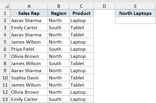
We want to count how many orders were Laptops sold in the North region.
Here is the formula:
=COUNTIFS(B2:B13,"North",C2:C13,"Laptop")
This returns 5.
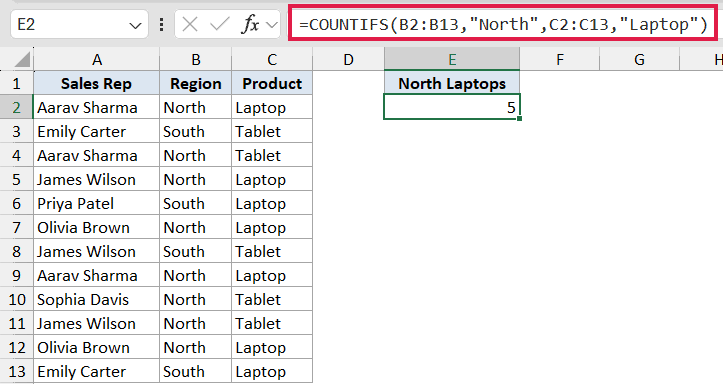
The formula uses two range and criteria pairs. A row only counts when BOTH conditions are true, meaning the Region is North AND the Product is Laptop.
Notice the text criteria are wrapped in quotes. That is how Excel knows you are matching against the words “North” and “Laptop”.
Example 2: Count Text Plus a Number
Next, let’s mix a text condition with a number condition.
This table has Customer in column A, Status in column B, and Amount in column C, across rows A2:C13. The statuses are Shipped, Pending, and Cancelled.
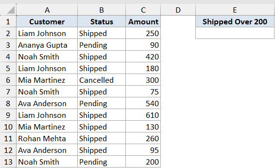
We want to count how many orders were shipped AND over 200.
Here is the formula:
=COUNTIFS(B2:B13,"Shipped",C2:C13,">200")
This returns 4.
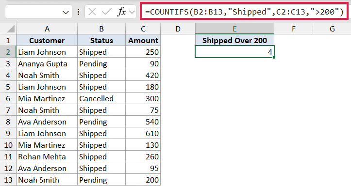
You can freely mix a text condition with a numeric comparison in the same COUNTIFS. The first pair checks for “Shipped”, and the second pair checks the amount.
The comparison goes in quotes too, written as “>200”. COUNTIFS reads that as “greater than 200”.
Example 3: Count Values Between Two Numbers
Now let’s count values that sit inside a range.
This dataset has Student in column A and Score in column B, across rows A2:B13.
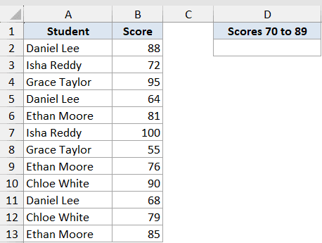
We want to count how many scores fall between 70 and 89, inclusive.
Here is the formula:
=COUNTIFS(B2:B13,">=70",B2:B13,"<=89")
This returns 6.
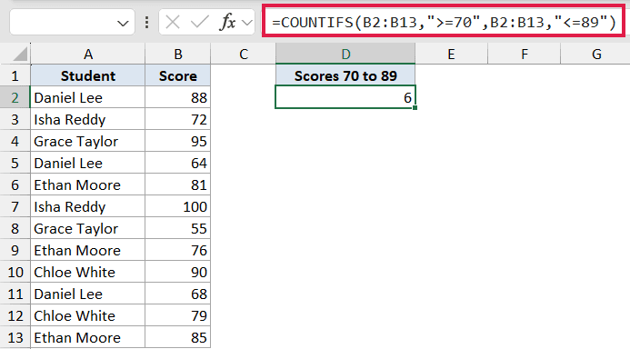
To count a range of values, you apply two conditions to the SAME column. One condition sets the lower bound and the other sets the upper bound.
Since both conditions have to be true at the same time, only scores from 70 up to 89 get counted.
Example 4: Count Within a Date Range
The same idea works nicely with dates.
Here we have Ticket ID in column A and Date in column B, across rows A2:B13. The dates run from January through April 2024.
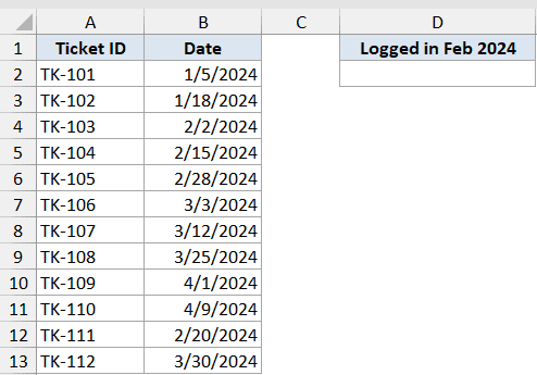
We want to count how many tickets were logged during February 2024.
Here is the formula:
=COUNTIFS(B2:B13,">="&DATE(2024,2,1),B2:B13,"<="&DATE(2024,2,29))
This returns 4.
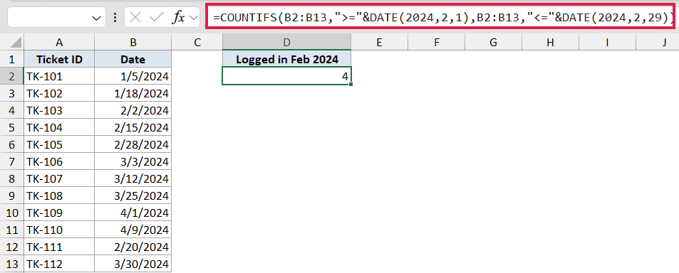
This is the same two-conditions-on-one-column trick, this time used on a date column. One condition is the start of February and the other is the end.
Using DATE() avoids regional date-format headaches, and the operator joins to it with the & symbol. So “>=”&DATE(2024,2,1) reads as “on or after Feb 1, 2024”.
Example 5: Count Using Conditions From Cells
Hard-coding conditions is fine, but pulling them from cells is more flexible.
This table is the same shape as Example 2, with Customer in A, Status in B, and Amount in C across A2:C13. Cell E2 holds the text “Shipped” and cell F2 holds the number 200.
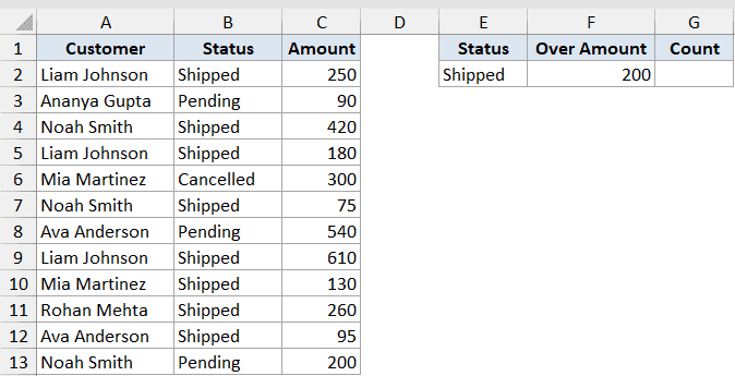
We want to count shipped orders above the amount typed in F2, using the conditions sitting in cells E2 and F2.
Here is the formula:
=COUNTIFS(B2:B13,E2,C2:C13,">"&F2)
This returns 4.
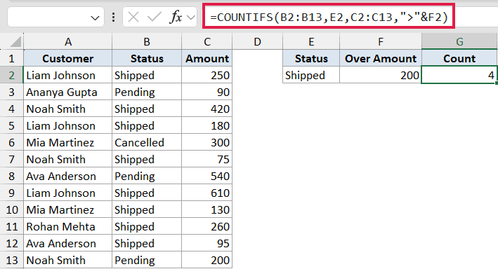
A plain cell reference like E2 works directly for the text condition. COUNTIFS reads the value in that cell and matches against it.
For the numeric comparison, keep the operator in quotes and join the cell with &, written as “>”&F2. Change E2 or F2 and the count updates on its own.
Pro Tip: A bare cell reference works as an “equals” criterion, but the moment you need >, <, or <>, the operator has to be in quotes and joined to the cell with &.
Example 6: Count Each Product for One Region
Now for the dynamic-array version, where one formula counts every category.
This table matches Example 1, with Sales Rep in A, Region in B, and Product in C across A2:C13. A small summary sits to the right: cell E2 holds =UNIQUE(C2:C13) which spills the distinct products down E2:E3 (Laptop, Tablet), and cell F2 holds the COUNTIFS below.
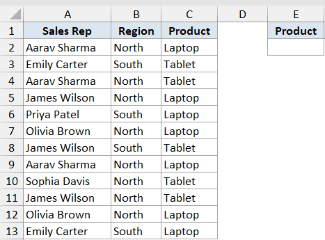
We want a North-region count for every product in one go.
Here is the formula:
=COUNTIFS(B2:B13,"North",C2:C13,E2#)
This spills 5 and 3.
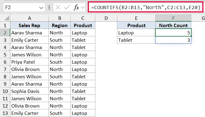
First, =UNIQUE(C2:C13) spills the distinct product list into E2:E3. Then COUNTIFS gets that spilled list as its second criterion using the # spill reference, written as E2#, so it returns a North count for each product and spills the results down.
One thing worth noticing is the asymmetry. The spilled list goes in the criteria slot, not the criteria-range slot. The criteria ranges stay fixed at B2:B13 and C2:C13.
Tips and Common Mistakes
- Every criteria range must have the same number of rows, or COUNTIFS returns a #VALUE! error.
- COUNTIFS uses AND logic. For OR logic, add two COUNTIFS together, or wrap one in SUM with an array constant like SUM(COUNTIFS(range,{“a”,”b”})).
- Wrap text and operators in quotes, and join cell references with & when you need a comparison.
- COUNTIFS is not case-sensitive, so “north” and “North” are treated the same.
- Use COUNTIF instead when you only have a single condition to check.
Once you get the hang of pairing each range with its own condition, COUNTIFS handles almost any “how many rows match all of this” question. Start with two text conditions, then layer on numbers, dates, and cell references. Try the examples on your own data and it falls into place quickly.
Related Excel Functions / Articles:
- COUNTIF Function in Excel
- SUMIFS Function in Excel
- COUNT Function in Excel
- SUMIF Function in Excel
- COUNTA Function in Excel
- IF Function in Excel
- Count the Number of Yes in Excel (Using COUNTIF)
- How to COUNTIF Partial Match in Excel?
- SUMPRODUCT vs SUMIFS Function in Excel
- How to Count Cells with Text in Excel?
