If you want to find the smallest number in a range, like the lowest price, the fastest time, or the coldest day, the MIN function is what you reach for.
It takes a range or a list of numbers and hands back the lowest one. MIN returns a single value, but it works happily inside dynamic array formulas like =MIN(FILTER(...)) when you need the smallest number from a filtered subset.
In this article, I’ll walk you through how MIN works with six practical examples.
MIN Function Syntax in Excel
The MIN function has a simple structure.
=MIN(number1,[number2],...)
- number1 – The first number, cell reference, or range you want to check.
- [number2], … – Optional. More numbers or ranges to include. You can add up to 255 arguments in total.
MIN looks across everything you give it and returns the lowest number. It ignores text, logical values, and empty cells inside a range.
When to Use MIN Function
Here are a few common situations where MIN comes in handy:
- Finding the lowest value in a list, such as the cheapest item or the minimum stock level.
- Pulling the best (lowest) time or score from a set of results.
- Spotting the earliest date in a range, since dates are stored as numbers.
- Getting the smallest value that meets a condition, when paired with IF or FILTER.
- Building a quick min-max summary at the top or bottom of a report.
Example 1: Find the Lowest Temperature
Let’s start with the simplest case.
Below is a dataset with the days of the week in column A and the recorded temperature in Fahrenheit in column B.
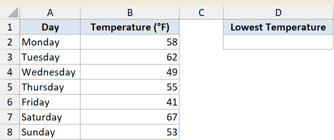
I want to know the lowest temperature across the whole week.
Here is the formula:
=MIN(B2:B8)

MIN scans every value in B2:B8 and returns 41, the temperature recorded on Friday. That’s all there is to a basic MIN. Point it at a range and it gives you the smallest number in it.
Example 2: Lowest Price Across Two Columns
Here’s a slightly bigger scenario.
This dataset lists grocery items in column A, with each item’s price at Store A in column B and Store B in column C.
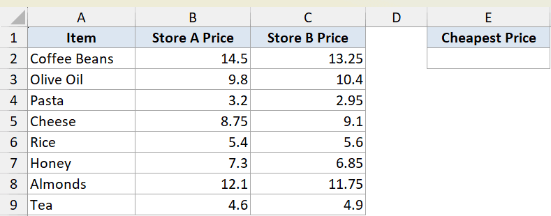
I want the single cheapest price anywhere in the table, no matter which store or item it belongs to.
Here is the formula:
=MIN(B2:B9,C2:C9)
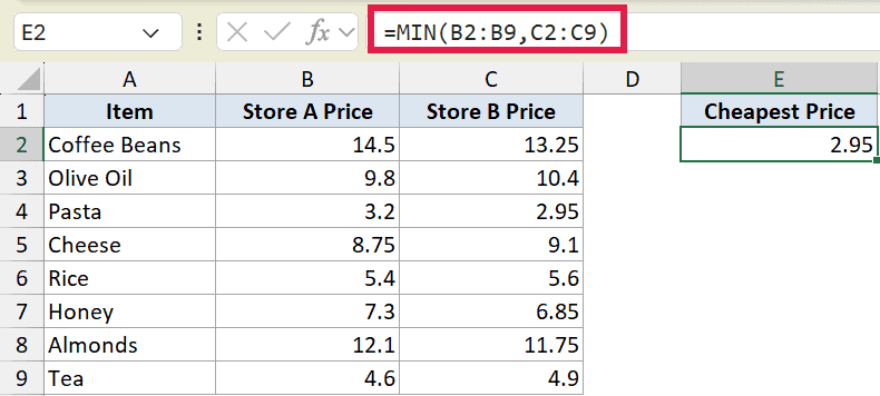
You can feed MIN more than one range by separating them with commas. Here it looks across both price columns at once and returns 2.95, the price of pasta at Store B.
Pro Tip: You can pass MIN up to 255 separate arguments, so you can mix ranges, single cells, and even typed-in numbers in the same formula.
Example 3: Best Time For Each Runner
Now let’s get a result for every row instead of one overall answer.
This dataset has runners in column A and their finish times for three races in columns B, C, and D.
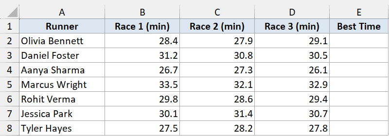
I want each runner’s best time, which is their lowest time across the three races.
Here is the formula:
=MIN(B2:D2)
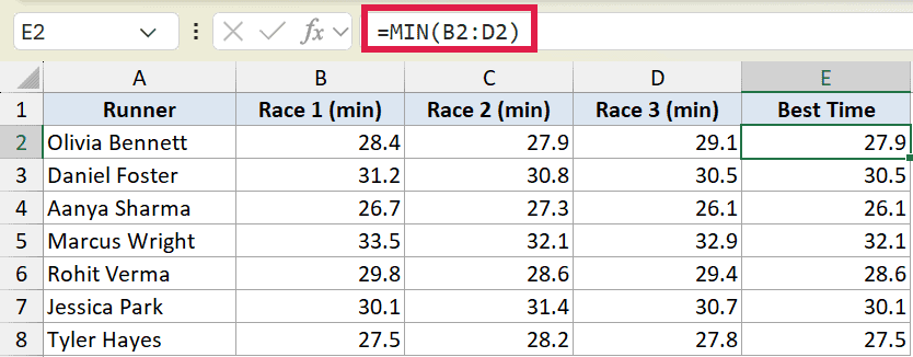
This formula sits in E2 and checks only that row’s three race times. For Olivia, it returns 27.9.
Copy it down column E and every runner gets their own best time, since the range shifts with each row.
Example 4: How MIN Handles Text and Blanks
This one shows what MIN does when a range isn’t all numbers.
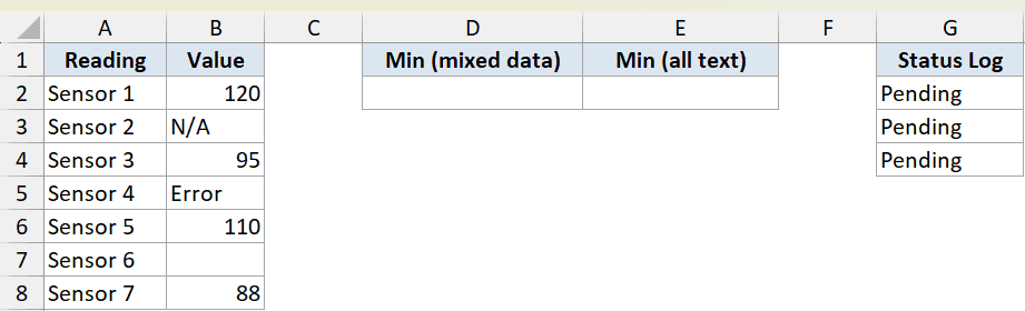
Column B holds sensor readings, but some cells contain text like “N/A” and “Error”, and one cell is blank. Column G holds three “Pending” status notes, with no numbers at all.
First, let’s find the minimum of the mixed column B, where numbers and text sit side by side.
Here is the formula:
=MIN(B2:B8)
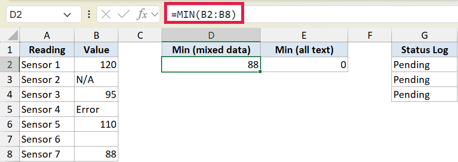
MIN simply skips the text and the blank cell and returns 88, the lowest actual number. You don’t have to clean the column first.
Now let’s see what happens when a range has no numbers at all.
Here is the formula:
=MIN(G2:G4)
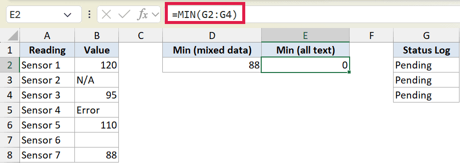
With nothing numeric to work with, MIN returns 0 instead of an error. That’s worth remembering, because a stray 0 in your report might mean “no numbers found” rather than an actual lowest value of zero.
Pro Tip: If you need MIN to count text or logical values as zeros instead of ignoring them, use MINA. For most everyday work, the standard MIN behavior of skipping text is what you want.
Example 5: Lowest Value With a Condition
Often you don’t want the overall minimum, you want the minimum for one category.
This dataset lists products in column A, their category in column B, and their price in column C.
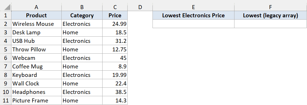
I want the lowest price among the Electronics products only.
The cleanest way to do this in modern Excel is MINIFS. Here is the formula:
=MINIFS(C2:C11,B2:B11,"Electronics")
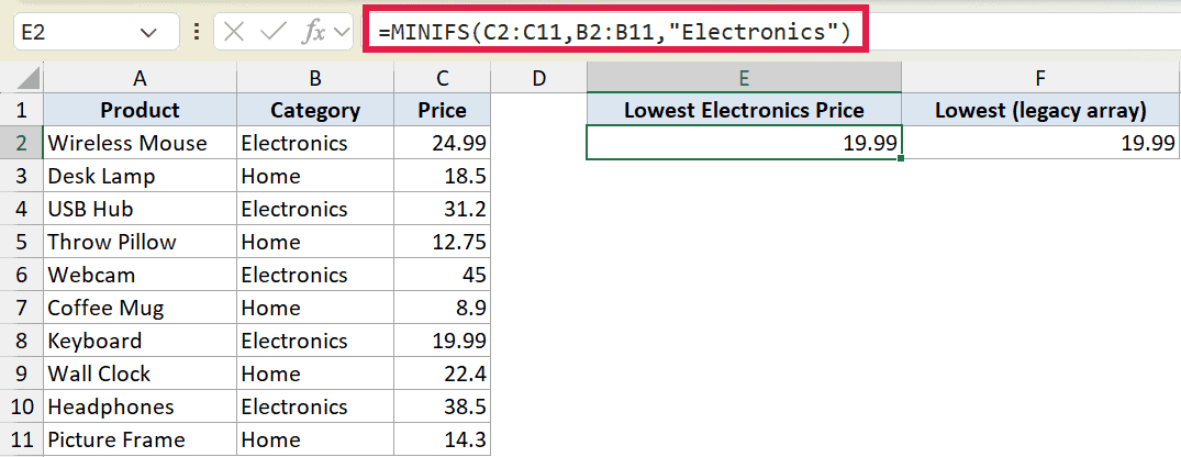
MINIFS reads as “give me the minimum of the price column, where the category column equals Electronics.” It returns 19.99, the price of the keyboard.
If you’re on an older version without MINIFS, you can get the same answer with MIN and IF. Here is the formula:
=MIN(IF(B2:B11="Electronics",C2:C11))
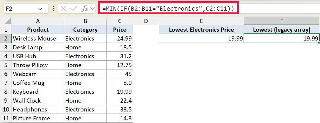
The IF part keeps only the Electronics prices and MIN finds the lowest of those. It also returns 19.99. In Excel 365 this works as a normal formula. In older versions you’d enter it with Ctrl+Shift+Enter as an array formula.
Pro Tip: MINIFS arrived in Excel 2019 and 365, and it’s much easier to read and maintain than the MIN(IF(…)) array trick. Reach for MINIFS first if your version has it.
Example 6: Smallest Value From a Filtered Set
For the last example, let’s combine MIN with a dynamic array function.
This dataset has order IDs in column A, the region for each order in column B, and the order value in column C.
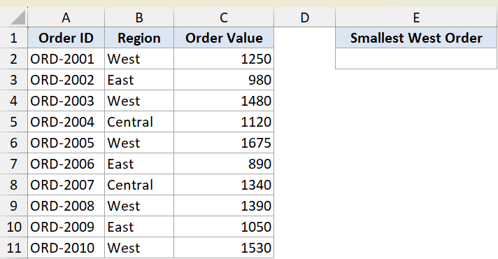
I want the smallest order value from the West region.
Here is the formula:
=MIN(FILTER(C2:C11,B2:B11="West"))
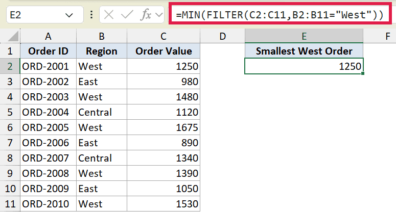
The FILTER function pulls out just the West region order values, and MIN takes the lowest from that smaller set. The result is 1250.
This is handy because FILTER builds the subset on the fly. MIN doesn’t spill on its own, but it works cleanly on the array that FILTER hands it.
Tips & Common Mistakes
- MIN ignores text, logical values, and blank cells inside a range, so you don’t need to clean your data before using it.
- An all-text or empty range returns 0, not an error. Don’t mistake that 0 for a real lowest value.
- MIN works on dates too, since dates are stored as serial numbers. The earliest date is the lowest number, so MIN gives you the oldest date.
- For a conditional minimum, use MINIFS on Excel 2019 or 365 instead of the older MIN(IF(…)) array formula.
- Don’t confuse MIN with SMALL. MIN gives you the lowest value, while SMALL lets you pull the 2nd lowest, 3rd lowest, and so on.
MIN is one of those functions you’ll use all the time. Point it at a range and it returns the smallest number, skipping any text or blanks along the way. It pairs nicely with MAX and AVERAGE in a quick summary row.
Pair it with MINIFS for conditional lows, or wrap it around FILTER when you need the minimum of a subset.
Related Excel Functions / Articles: