If you want to find the middle value in a list of numbers, the one where half the values sit above it and half below, the MEDIAN function is what you’re looking for.
It’s a great way to summarize data when a few unusually high or low numbers would throw off the average. In this article, I’ll show you how to use MEDIAN with several practical examples.
MEDIAN returns a single value, but it works seamlessly inside dynamic array formulas like =MEDIAN(FILTER(...)).
MEDIAN Function Syntax in Excel
The MEDIAN function returns the middle number from a set of values.
=MEDIAN(number1, [number2], ...)
- number1 – The first number, cell reference, or range you want the median of. This one is required.
- number2, … – Additional numbers or ranges. These are optional, and you can add up to 255 of them.
When to Use MEDIAN Function
- When you want a “typical” value that isn’t skewed by a few very high or very low numbers.
- When summarizing salaries, prices, or response times, where outliers are common.
- When comparing the median against the average to spot skew in your data.
- When you need the middle value across several separate ranges in one go.
Example 1: Find the Median of a Column
Let’s start with a simple example.
Below is the dataset. It has a list of employees in column A and their salaries in column B.
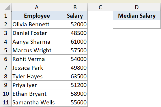
I want to find the median salary across all ten employees.
Here is the formula:
=MEDIAN(B2:B11)
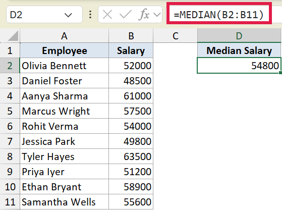
This returns 54800. MEDIAN sorts the ten salaries internally and, since there’s an even count, it averages the two middle values to get the result.
You don’t need to sort the data yourself. MEDIAN handles that for you no matter what order the numbers are in.
Example 2: Median vs Average
Here’s a practical scenario that shows why median is often more useful than average.
Below is the same kind of dataset, employees in column A and salaries in column B. This time one person earns far more than the rest.
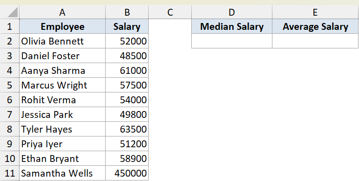
I want to compare the median salary against the average salary for this group.
Here is the formula for the median:
=MEDIAN(B2:B11)
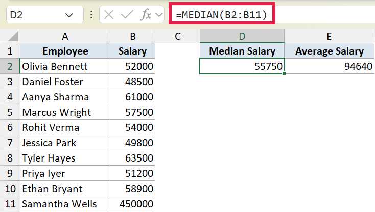
The median comes out to 55750, right in the middle of the typical salaries.
And here is the average for comparison:
=AVERAGE(B2:B11)
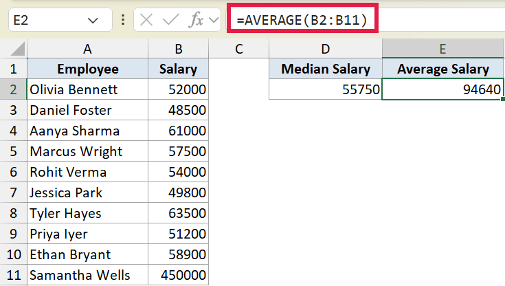
The average jumps to 94640, way above what almost everyone actually earns.
That gap is the whole point. One salary of 450000 drags the average up, but the median barely moves. When your data has outliers, the median gives a far more honest picture of the typical value.
Example 3: Blanks Skipped, Zeros Counted
Let’s look at how MEDIAN treats empty cells and zeros, because they behave differently.
Below is the dataset. Column A has order IDs and column B has delivery times in hours. Two rows are blank, and two orders were delivered in 0 hours.
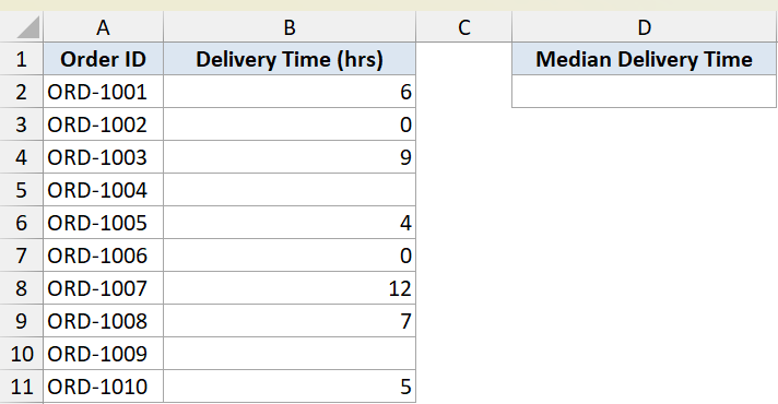
I want the median delivery time across the orders that actually have a recorded time.
Here is the formula:
=MEDIAN(B2:B11)
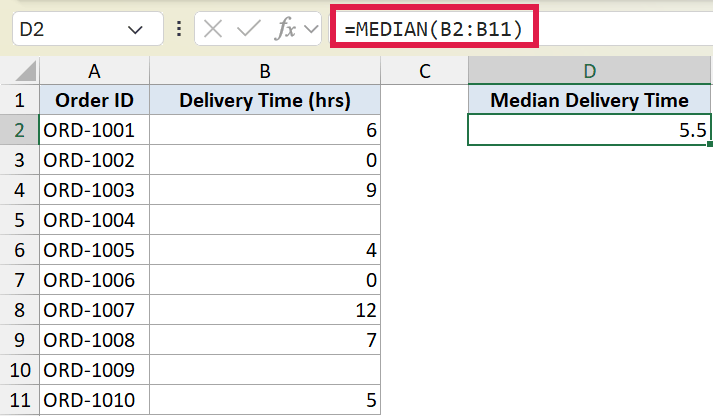
This returns 5.5. MEDIAN ignored the two blank cells completely, so only eight values went into the calculation.
But the two zeros were counted as real values of 0. With an even count of eight, MEDIAN averaged the two middle numbers, 5 and 6, to give 5.5.
Pro Tip: A blank cell and a cell with 0 are not the same to MEDIAN. Blanks are skipped, but zeros count as actual values and can pull the median down. If a 0 really means “no data,” leave the cell empty instead.
Example 4: Median for a Specific Category
Here’s a scenario where you want the median for just one group inside a larger table.
Below is the dataset. Column A has order IDs, column B has the region, and column C has delivery times in hours.
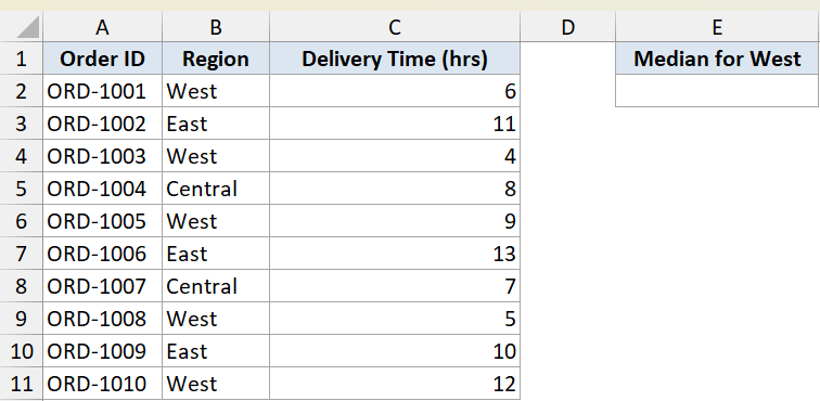
I want the median delivery time for orders in the West region only.
Here is the formula:
=MEDIAN(FILTER(C2:C11,B2:B11="West"))
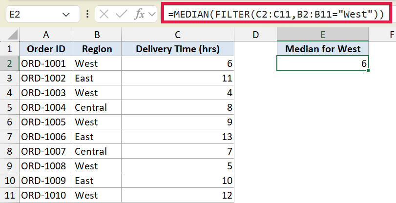
This returns 6. FILTER first pulls out only the delivery times where the region is “West,” then MEDIAN finds the middle value of that filtered set.
MEDIAN doesn’t have a built-in criteria argument like SUMIF does, so wrapping it around FILTER is the cleanest way to get a conditional median in Excel 365. If you need more methods, including ones that work in older Excel versions, see our full guide on the median if in Excel.
Example 5: Median Across Multiple Ranges
Let’s finish with an example that uses more than one range in a single MEDIAN call.
Below is the dataset. Column A has products, column B has Q1 units sold, and column C has Q2 units sold.
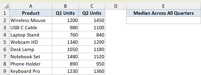
I want the median units sold across both quarters combined.
Here is the formula:
=MEDIAN(B2:B9,C2:C9)
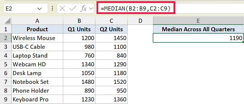
This returns 1190. MEDIAN pools all sixteen values from both columns into one set, then finds the middle.
You can pass MEDIAN as many separate ranges as you need, and it treats them all as one combined pool. The ranges don’t have to be next to each other on the sheet.
Tips & Common Mistakes
- MEDIAN ignores text, blank cells, and logical values (TRUE/FALSE) in a referenced range. They simply don’t get counted.
- Zeros are different. A 0 is a real number to MEDIAN and goes into the calculation, so don’t confuse an empty cell with a cell holding 0.
- When there’s an even number of values, MEDIAN averages the two middle ones. So the result can be a number that doesn’t actually appear in your data, like 5.5 or 54800.
- Median is your friend when data is skewed. If a handful of very large or very small values are distorting the average, switch to MEDIAN for a more representative figure.
- To see the mean, median, and mode side by side for the same data, try our mean median mode calculator. It’s a quick way to compare all three at once.
- If you want to go beyond the middle and see how your values spread out, the QUARTILE.INC function splits your data into four equal parts.
MEDIAN is one of those functions that’s easy to use but earns its keep when your data is messy. You’ve now seen it on a single column, side by side with the average, dealing with blanks and zeros, pulling a conditional median through FILTER, and pooling several ranges into one result.
Try it on your own data and see how the median compares to the average. The difference often tells you a lot.
Related Excel Functions / Articles: