ABS Function in Excel (4 Easy Examples)

If you want to strip the negative sign off a number and keep only its size, the ABS function in Excel is what you reach for. It returns the absolute value, so -1450 and 1450 both come back as 1450.

In Excel 365, you can also feed ABS a range and the results spill into the cells below.

Table of Contents

ABS Function Syntax in Excel

The ABS function takes a single number and returns its distance from zero, with no sign attached.

=ABS(number)

number (required) is the value you want the absolute value of. This can be a typed number, a cell reference, or a formula that returns a number.

When to Use ABS Function

You want a variance or difference reported as a size, not a direction (forecast vs actual, budget vs spent).
You need to remove negative signs from a column of figures before charting or summing them.
You want to compare two numbers and only care how far apart they are.
You are measuring error or deviation, where the sign does not matter.

Example 1: Get the Absolute Value of a Number

Let’s start with the simplest case.

Below is the dataset. Column A holds a single account balance of -1450, and column B is where we will return its absolute value.

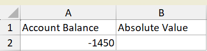
Abs example 1 dataset showing Account Balance -1450 in cell A2 and Absolute Value header in cell B1

We want to turn that -1450 into a plain positive 1450.

Here is the formula:

=ABS(A2)

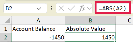
Excel formula bar showing =ABS(A2) to convert the negative value in cell A2 to a positive 1450 in cell B2

ABS looks at the value in A2, drops the minus sign, and returns 1450. A positive number passed to ABS comes back unchanged. If you instead want to flip signs the other way, see how to make positive numbers negative.

Pro Tip: ABS changes the value, not how it looks. If a result still shows in red or in parentheses, that is a number format on the cell, not the actual sign. Clear the accounting or custom format if you want the plain positive number to show.

Example 2: Absolute Difference Between Two Columns

Here’s a common one. You have a forecast and an actual figure, and you want the gap between them as a positive number.

Below is the dataset. Column A lists the month, column B the forecast, column C the actual, and column D is where the variance goes.

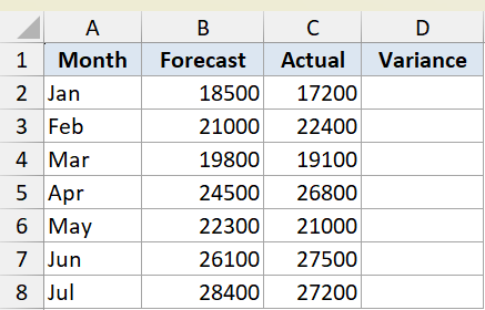
Excel dataset with columns for Month, Forecast, and Actual values from January to July for an ABS function example

We want the size of the difference in each row, whether the actual came in above or below the forecast.

Here is the formula:

=ABS(B2-C2)

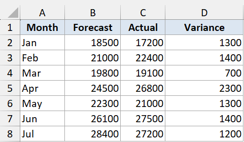
Excel table showing Month, Forecast, and Actual data with a Variance column calculated using the ABS function

Excel first works out B2 minus C2, then ABS removes the sign. So a forecast of 18500 against an actual of 17200 gives 1300, and a month that overshot gives a positive number too.

Copy the formula down the column and every row reports its gap as a positive figure. That makes the column easy to total or sort by size.

Example 3: Spill Absolute Values Across a Range

Let’s use a single formula to handle a whole column at once.

Below is the dataset. Column A holds a list of daily changes, some positive and some negative, and column B is empty.

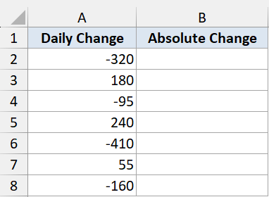
Excel dataset showing a Daily Change column with positive and negative values and an empty Absolute Change column

We want the absolute value of every daily change, without copying a formula down each row.

Here is the formula:

=ABS(A2:A8)

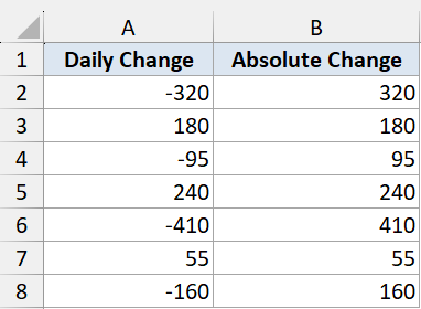
Excel table showing Daily Change in column A and the corresponding positive Absolute Change in column B

You type this once in B2 and it spills down through B8 on its own. Each cell shows the positive version of the matching value in column A.

This works in Excel 365 and Excel for the web. In older versions you would put =ABS(A2) in B2 and drag it down instead.

Pro Tip: If the spill formula returns a #SPILL! error, something is sitting in the cells where the results need to land. Clear B3:B8 so the formula has empty room to spill into.

Example 4: Sum of Absolute Differences with SUMPRODUCT

Here’s a neat one. Instead of adding a helper column, you can total all the absolute differences in a single cell.

Below is the dataset. Column A lists each item, column B the budget, and column C the amount spent. Cell E2 will hold the combined gap.

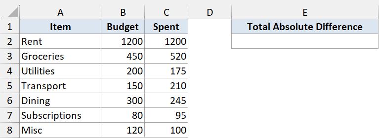
Excel dataset for ABS function with columns for Item, Budget, Spent, and Total Absolute Difference

We want the total of every absolute difference between budget and spent, across all seven items, in one formula.

Here is the formula:

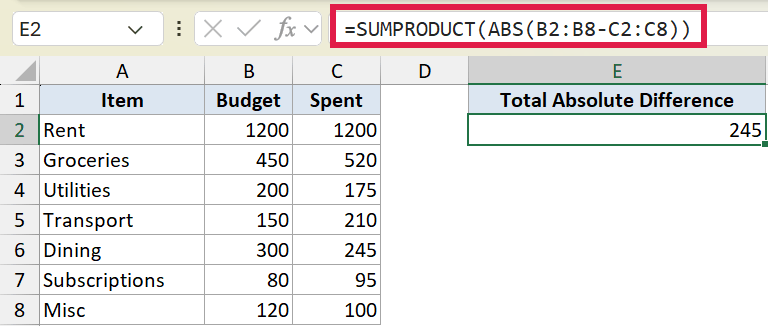
=SUMPRODUCT(ABS(B2:B8-C2:C8))

Excel formula =SUMPRODUCT(ABS(B2:B8-C2:C8)) calculating total absolute difference between budget and spent columns

How this formula works:

B2:B8-C2:C8 subtracts spent from budget for every row, giving an array of positive and negative gaps.
ABS turns each of those gaps into a positive number.
SUMPRODUCT adds the whole array up into one figure.

So you get the total over-and-under spend in a single cell, no helper column needed. ABS spills natively here, which is what lets SUMPRODUCT take the whole array in one pass.

Tips & Common Mistakes

ABS only takes one argument. Passing it a range like =ABS(A2:A8) works as a spill in 365, but if you need a single total use a wrapper such as SUMPRODUCT or SUM.
ABS changes the value, not the display. A cell that still looks negative is showing a number format (red text, parentheses), not a negative number. Clear the format to see the plain figure.
A #SPILL! error from =ABS(A2:A8) means the cells below are not empty. Clear the spill range and the results will fill in.
ABS has no modern replacement. It is a basic math function, and the only thing that has changed is that it now spills over a range in 365.

ABS is one of the simplest functions in Excel, but it pulls real weight whenever you care about size rather than sign. You have seen it on a single value, across a variance column, spilled over a whole range, and totaled inside SUMPRODUCT.

Pick the form that fits your sheet and you can drop negative signs in seconds.

List of All Excel Functions

Related Excel Functions / Articles: