How to Build a Mortgage Calculator in Excel

If you’re about to take on a home loan, you probably want to know the monthly payment before you sign anything. A mortgage is a big commitment, and the numbers a bank quotes rarely show how much goes to interest.

The good news is that Excel already has the functions for this, so you don’t need any add-ins. I’ll build a mortgage calculator step by step, from the input cells to the payment, a full amortization schedule, and monthly escrow contributions.

Step 1: Set Up the Mortgage Inputs

Every calculator starts with the numbers you can change. I’ll keep all the loan details in their own labeled cells so the rest of the sheet just points at them.

For this example I’m buying a home priced at $350,000 with a 20% down payment, financed at a 6.5% annual rate over 30 years. Putting these in one block makes it easy to swap in your own figures later.

Here are the input cells I set up:

1. In cell B1, enter the Home Price: 350000.
2. In cell B2, enter the Down Payment: 70000.
3. In cell B3, enter the Loan Amount as =B1-B2, which gives 280000.
4. In cell B4, enter the Annual Interest Rate (the loan’s note rate): 6.5%.
5. In cell B5, enter the Loan Term in years: 30.
6. In cell B6, enter the First Payment Date: 1-Aug-2026.

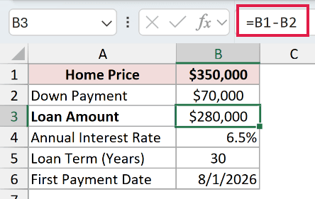
With the loan amount as a formula, changing the home price or the down payment updates everything downstream automatically. That’s the whole point of keeping inputs separate from calculations.

Note: Type the interest rate as 6.5% (with the percent sign) so Excel stores it as 0.065. If you type 6.5 on its own, the rate input is 100 times too large and the payment will be wrong. Use the loan’s note rate in B4. A mortgage APR can include points and fees, so it is not automatically the correct rate to divide by 12 for this schedule.

Step 2: Calculate the Monthly Payment With PMT

The PMT function does the core math for this fixed-rate loan. It returns a level payment based on a constant interest rate and constant payments. Because the optional type argument is omitted in this formula, Excel assumes payments are due at the end of each period.

Since a mortgage is paid monthly, I convert the annual rate to a monthly one and the term in years to a number of months right inside the formula.

Here is the formula I put in cell B8:

=PMT(B4/12,B5*12,-B3)

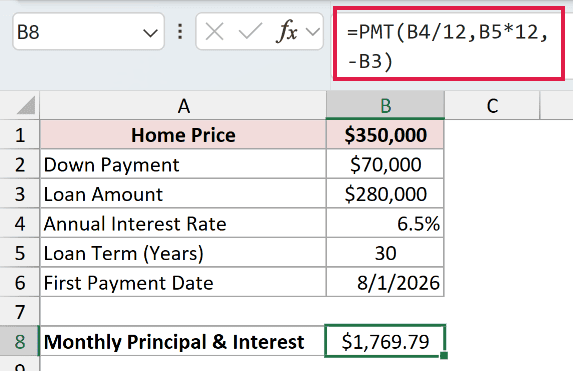
This returns $1,769.79, the fixed monthly principal-and-interest payment.

How does this formula work?

B4/12 turns the annual rate into a monthly rate, and B5*12 turns the 30-year term into 360 payments. I enter the loan as -B3 because PMT treats money you receive as positive and money you repay as negative, which flips the payment positive.

Note: This payment covers principal and interest only. Property taxes, homeowner’s insurance, and PMI are separate, and I’ll track monthly tax and insurance contributions in Step 4.

Step 3: Build the Amortization Schedule

The single payment number hides a lot. In the early years, most of each payment is interest, and only a little chips away at the balance. An amortization schedule shows that split for every month.

I’ll build a table with one row per payment. If you’d rather skip the build and get the same breakdown instantly, our loan amortization schedule calculator does it from three inputs.

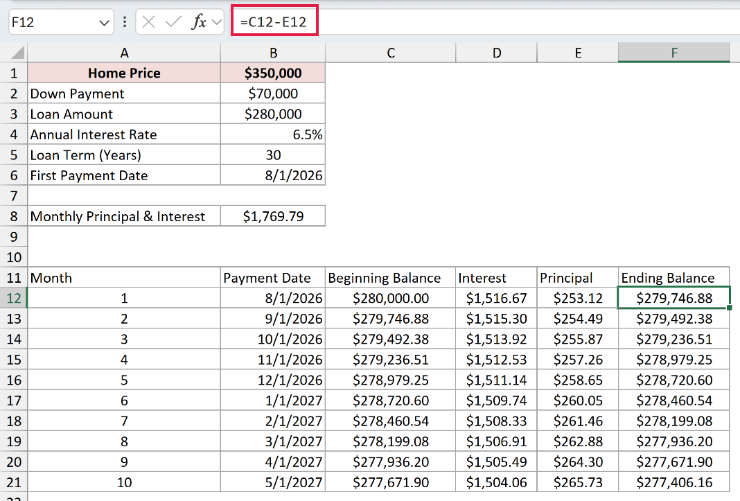
To do it yourself, set up these column headers in row 11: Month, Payment Date, Beginning Balance, Interest, Principal, Ending Balance.

Here are the steps to fill the first row of the schedule:

1. In the Month column, enter 1 for the first payment.
2. For the Payment Date, use =EDATE($B$6,A12-1) so the first row shows the start date and each later row steps forward one month.
3. For the Beginning Balance, point the first row at the loan amount with =$B$3.

Now for the interest and principal. IPMT returns the interest portion of a given payment, and PPMT returns the principal portion. They take the same arguments as PMT, plus the period number you want.

Here is the interest formula for the first row:

=IPMT($B$4/12,A12,$B$5*12,-$B$3)

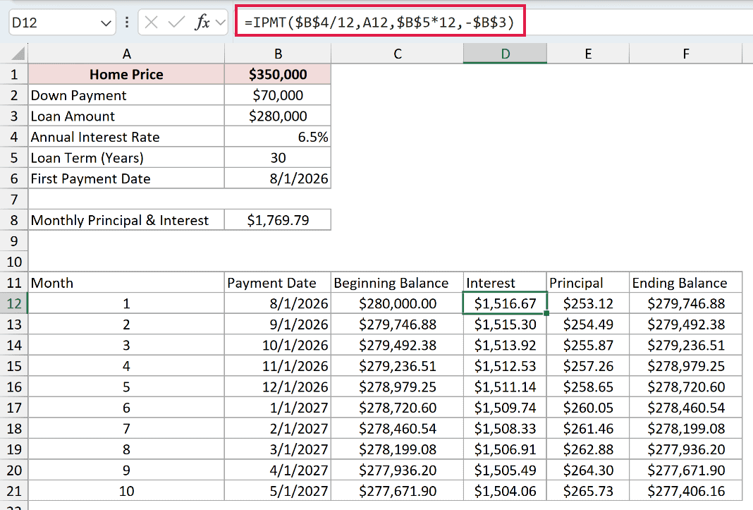
For month 1 this returns $1,516.67. Next to it, the principal formula uses PPMT:

=PPMT($B$4/12,A12,$B$5*12,-$B$3)

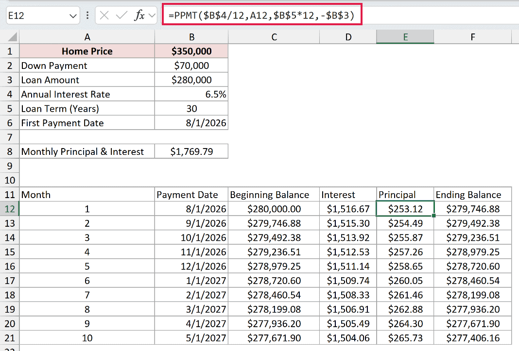
That returns $253.12, so on your very first payment only about $253 of the $1,769.79 actually reduces what you owe. The Ending Balance is just the beginning balance minus the principal you paid:

=C12-E12

Build row 13 as the second payment row before filling anything down:

1. In A13, enter =A12+1 for the next month number.
2. In B13, enter =EDATE($B$6,A13-1) for the next payment date.
3. In C13, enter =F12 so the beginning balance equals the prior ending balance.
4. In D13, enter =IPMT($B$4/12,A13,$B$5*12,-$B$3) for that month’s interest.
5. In E13, enter =PPMT($B$4/12,A13,$B$5*12,-$B$3) for that month’s principal.
6. In F13, enter =C13-E13 for the ending balance.

With row 13 complete, select A13:F13 and copy it down through row 371. That produces months 2 through 360, with each row carrying forward the prior ending balance.

How does this formula work?

The A12 in IPMT and PPMT is what makes each row unique. It tells Excel which payment number you’re on, so the interest shrinks and the principal grows as the balance falls. Everything else stays locked with $ signs.

Step 4: Add a Monthly Escrow Contribution Schedule

Most lenders collect property tax and insurance along with your payment and hold them in an escrow account. You can track how much you contribute each month next to the loan schedule.

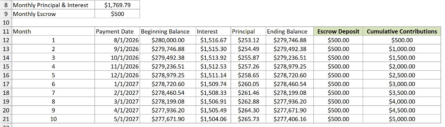
I’m estimating $4,200 a year in property tax and $1,800 in homeowner’s insurance, which is $6,000 a year, or $500 a month. Set up two columns beside the schedule: Escrow Deposit and Cumulative Contributions.

For this example, the estimated total monthly payment is $1,769.79 + $500 = $2,269.79. This excludes PMI, HOA dues, other fees, and future escrow changes.

Here are the steps to build the reserve columns:

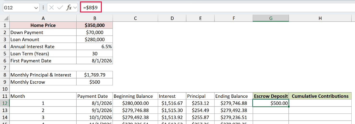
1. Put the monthly escrow amount in its own input cell, say B9, as 500.
2. In the first Escrow Deposit row, reference it with =$B$9 so every month deposits the same amount.

The Cumulative Contributions column is a running total. The first row equals the first deposit, and every row after adds the new deposit to the previous total.

Here is the cumulative-contributions formula for the second row:

=H12+G13

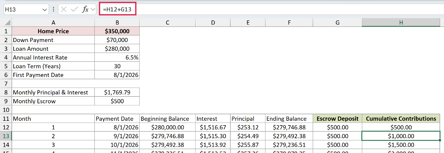
Here H12 is the prior cumulative total and G13 is this month’s deposit. Copy it down alongside the loan schedule to see how much you have contributed.

This is not the actual escrow account balance because it does not subtract tax and insurance disbursements. To model that balance, add those withdrawals in the months when the lender pays the bills.

Step 5: Summarize Total Interest and Payoff Date

The schedule already has every number you need, so the summary is just a few totals pulled from it. This is where the true cost of the loan shows up.

To total the interest paid over the life of the loan, sum the entire Interest column:

=SUM(D12:D371)

For this loan that comes to $357,124.57 in interest, on top of the $280,000 borrowed. The total principal and interest paid is $637,124.57, which is why the interest column is worth seeing.

For the payoff date, count forward the full term from your first payment:

=EDATE(B6,B5*12-1)

Starting on 1-Aug-2026, the loan is paid off on 1-Jul-2056. You can confirm it by checking that the Ending Balance in the last row of the schedule reads $0.

Additional Notes About Building a Mortgage Calculator in Excel

• PMT, IPMT, and PPMT assume a constant rate and constant payments. For an adjustable-rate mortgage, each rate reset requires you to recalculate the payment from the remaining balance, new rate, and remaining term, then calculate interest from the current balance. Simply changing the original rate argument partway down the existing IPMT/PPMT schedule gives the wrong result.
• Keep every rate and term as a reference to an input cell, never a hard-coded number in the formula. That way you can test a 15-year term or a lower rate by changing one cell.
• Format the payment, balance, and interest cells as currency and the rate as a percentage. It won’t change the math, but it makes the sheet far easier to read.
• The escrow figure is an estimate. Tax rates and insurance premiums change over time, so revisit the $500 monthly deposit once a year.

Frequently Asked Questions

How do I add extra monthly payments to see the loan pay off sooner?

Do not keep using the original IPMT and PPMT schedule after an extra principal payment. Rebuild that version from the balance in each row.

Add Planned Extra Principal in column J and Applied Extra Principal in column K. Use =C12*$B$4/12 for Interest, =MIN(C12,MAX(0,$B$8-D12)) for Scheduled Principal, and =MIN(J12,MAX(0,C12-E12)) in K12 to cap the extra principal.

Then use =MAX(0,C12-E12-K12) for Ending Balance. The next row begins with the prior Ending Balance, so future interest falls correctly and the balance never goes below zero.

Can I build this calculator on Excel for Mac or the web version?

Yes. PMT, IPMT, PPMT, EDATE, and SUM are supported in current Excel for Mac and Excel for the web, so these formulas use the same A1 references there. Date and currency display may follow your regional settings.

Why does my payment come out negative?

That happens when the loan amount is entered as a positive number inside PMT. Enter it as a negative, like -B3, or wrap the whole formula in a minus sign to flip the result.

Conclusion

This calculator combines the monthly principal-and-interest payment, amortization schedule, escrow contribution estimate, and payoff summary in one sheet. I hope you found this article helpful!

Other Excel articles you may also like:

• NPER Function in Excel
• PV Function in Excel
• FV Function in Excel