
Excel’s PPMT function returns the principal portion of a payment for a specified period, assuming constant payments and a constant interest rate.
It shows how much of a loan payment reduces the balance. Pair it with IPMT to separate the principal and interest portions of the same payment.
In this article, I’ll show you how to build principal repayment schedules, separate principal from interest, and compare different payment timings.
PPMT Function Syntax in Excel
The PPMT function uses the following syntax:
=PPMT(rate, per, nper, pv, [fv], [type])
rateis the required interest rate for each period.peris the required payment period. It must be from 1 throughnper.nperis the required total number of payment periods.pvis the required present value, such as the original loan balance.fvis the optional balance after the final payment. Excel uses 0 when you omit it.typeis optional. Use 0 or omit it for end-of-period payments, and use 1 for beginning-of-period payments.
When to Use PPMT Function
- Show the principal repaid in each loan period.
- Separate a payment into principal and interest.
- Total the principal repaid over a selected period range.
- Model financing with a final balance or buyout.
Example 1: Create a Principal Repayment Schedule
Let’s start with the first year of a fixed-rate loan.
Below is the dataset with payment numbers 1 through 12 and an empty principal-repaid column.
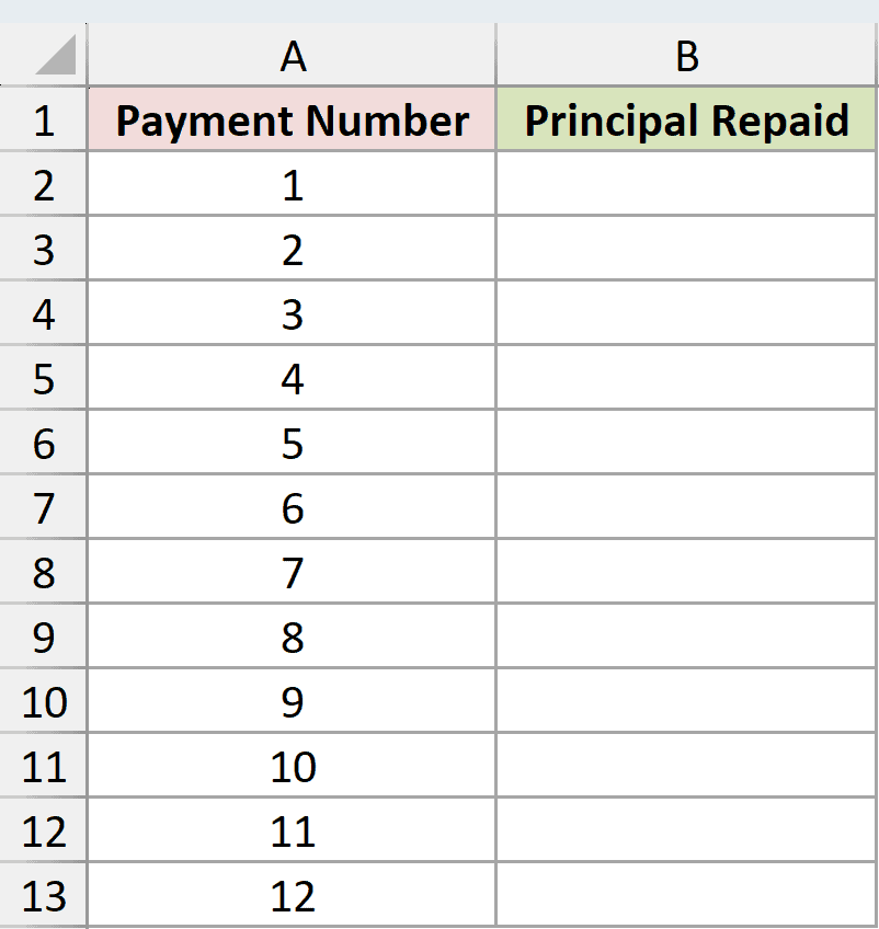
I want to calculate the principal portion of each payment for an $18,000 loan at 6.5% over 60 months.
Here is the formula:
=-PPMT(6.5%/12,A2:A13,60,18000)
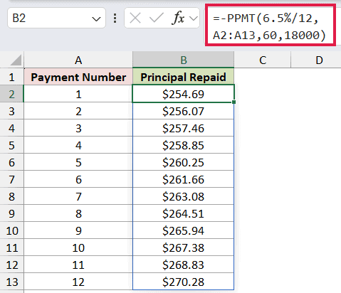
The annual rate is divided by 12 because the payments are monthly. The range A2:A13 supplies all 12 payment numbers, so one formula spills the schedule.
PPMT returns payments as negative cash flows. The leading minus sign displays them as positive amounts, from $254.69 in month 1 to $270.28 in month 12.
Example 2: Split Principal and Interest
PPMT is easiest to understand beside the other parts of a loan payment.
Below is a $15,000 loan at 7.2% for 36 months, with payment number 18 selected.
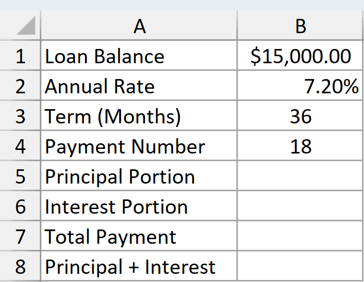
I want to calculate the principal and interest portions, then confirm that they add up to the full payment.
Here is the principal formula:
=-PPMT(B2/12,B4,B3,B1)
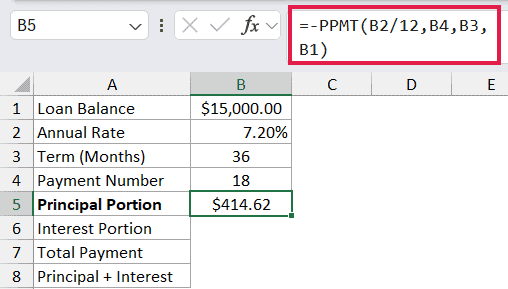
PPMT returns $414.62 as the principal portion of payment 18.
Here is the interest formula:
=-IPMT(B2/12,B4,B3,B1)
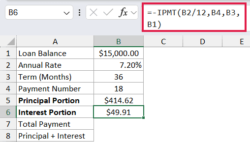
The IPMT function returns $49.91 as the interest portion.
Here is the full payment formula:
=-PMT(B2/12,B3,B1)
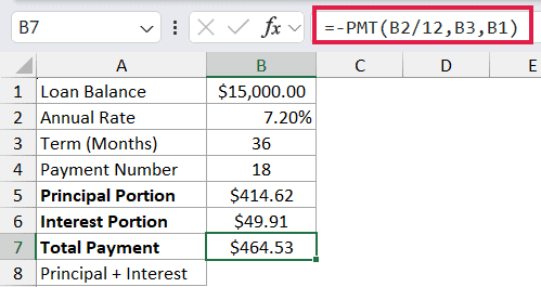
The PMT function returns the full payment of $464.53.
Here is the reconciliation formula:
=B5+B6
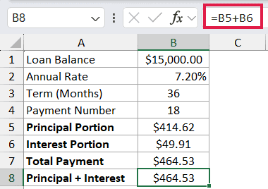
Adding $414.62 of principal and $49.91 of interest also gives $464.53. The two parts match the full payment exactly.
Example 3: Total Principal Over Several Periods
You can combine PPMT with a generated list of periods to get a cumulative amount.
Below is a seven-year equipment loan for $42,000 at 6.25%, with periods 1 through 12 selected.
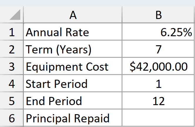
I want to calculate the total principal repaid during the first 12 monthly payments.
Here is the formula:
=-SUM(PPMT(B1/12,SEQUENCE(B5-B4+1,1,B4),B2*12,B3))
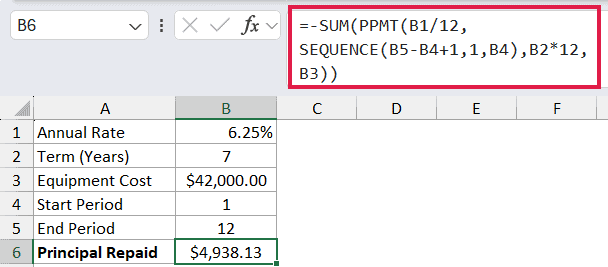
The SEQUENCE function creates payment numbers 1 through 12. PPMT returns the principal for each number, and the SUM function combines those values.
The leading minus sign turns the negative cash-flow result into a positive total of $4,938.13.
CUMPRINC is more direct when you need only the period total: =-CUMPRINC(B1/12,B2*12,B3,B4,B5,0). PPMT remains useful when the same model also needs period-by-period amounts.
Example 4: Include an End-of-Term Buyout
The optional fv argument can represent a balance left after the scheduled payments.
Below is equipment financing with an 8% annual rate, 48 monthly periods, a $36,000 price, and a $5,000 buyout.
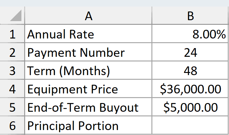
I want the principal portion of payment 24 while the financing still leaves the buyout at the end.
Here is the formula:
=-PPMT(B1/12,B2,B3,B4,-B5,0)
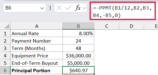
The future value is -B5 because the $5,000 buyout is cash paid at the end. The formula returns $640.97 as the principal portion of payment 24.
The final 0 sets payments at the end of each month. Omitting type would give the same result.
Example 5: Compare Payment Timing
The type argument changes the principal schedule when payments occur at the beginning instead of the end of each period.
Below is a $28,000 loan at 7% for 48 months, with payment number 6 selected.
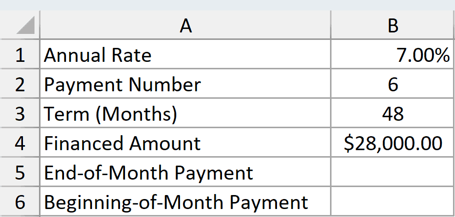
I want to compare the principal portion for end-of-month and beginning-of-month payments.
Here is the end-of-month formula:
=-PPMT(B1/12,B2,B3,B4,0,0)
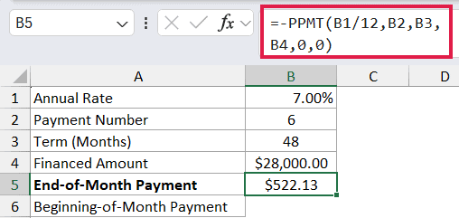
With type set to 0, payment 6 includes $522.13 of principal.
Here is the beginning-of-month formula:
=-PPMT(B1/12,B2,B3,B4,0,1)
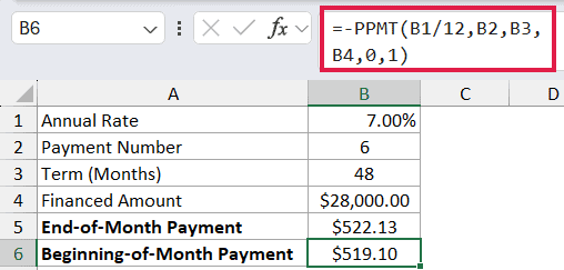
With type set to 1, the principal portion is $519.10. The payment timing changes the balance before interest is calculated, so the schedule changes too.
Pro Tip: Use the same type value in PPMT, IPMT, and PMT when you reconcile payment components. Mixing beginning-of-period and end-of-period assumptions makes the comparison invalid.
Example 6: Calculate Principal for Multiple Loans
PPMT can spill across aligned ranges, not just a list of periods for one loan.
Below is the dataset with six accounts, each with its own balance, annual rate, term, and selected payment number.
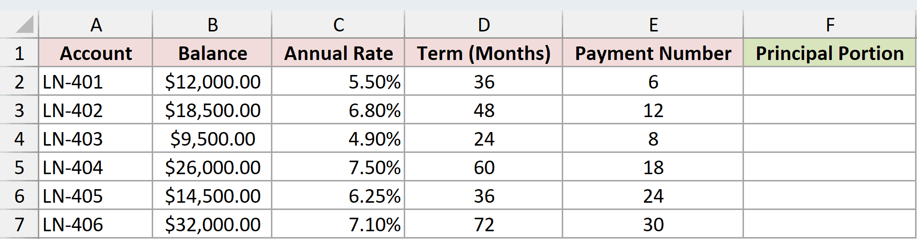
I want to calculate the principal portion for every account with one formula.
Here is the formula:
=-PPMT(C2:C7/12,E2:E7,D2:D7,B2:B7)
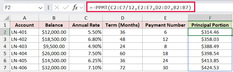
Each argument uses the values from the same row. For example, LN-401 uses its 5.5% rate, 36-month term, $12,000 balance, and payment number 6.
The formula spills six principal amounts, from $314.46 for LN-401 to $424.53 for LN-406.
Tips & Common Mistakes
- Keep
rateandnperin matching units. For monthly payments, divide an annual rate by 12 and use the total number of months. - Keep
perbetween 1 andnper. - PPMT normally returns a negative number for a payment. Add a leading minus sign when you want to display principal repaid as a positive amount.
- Excel uses 0 for
fvandtypewhen you omit them. - Microsoft lists PPMT for Excel 2016 and later.
- In Excel 365, PPMT spills when
peror aligned arguments are ranges. A blocked output area returns#SPILL!, while implicit intersection reduces the formula to one result. - In older Excel versions without dynamic arrays, use one PPMT formula per row and copy it down.
I’ve shown you how PPMT builds principal schedules, reconciles payment components, totals selected periods, and handles buyouts and payment timing. I hope you found this article helpful.
Related Excel Functions / Articles:
Other Excel articles you may also like:
