If you want to figure out what a future stream of money is worth in today’s dollars, the PV function is what you’re looking for.
It works for loans, annuities, retirement payouts, and one-time future amounts. As long as the interest rate and payment schedule stay constant, PV gives you the lump-sum value as of today.
PV returns a single value, but it works just fine inside dynamic array formulas like =PV(B2#, C2#, D2#) when you want to evaluate multiple scenarios in one shot.
In this article, I’ll walk you through the syntax, the sign convention quirk that trips people up, and a few practical examples.
PV Function Syntax
Here is the syntax of the PV function:
=PV(rate, nper, pmt, [fv], [type])
- rate – The interest rate per period. If your loan has an annual rate but monthly payments, divide the annual rate by 12.
- nper – The total number of payment periods. For a 5-year loan with monthly payments, this is 60.
- pmt – The payment made each period. It stays the same across all periods. Enter outflows as negative numbers.
- fv – Optional. The future value or cash balance you want after the last payment. Defaults to 0 if you skip it.
- type – Optional. Set to 0 (or skip) if payments are made at the end of each period, or 1 if they’re made at the beginning.
A quick heads-up on the sign convention.
Excel treats money you pay out as negative and money you receive as positive.
So if you’re calculating the present value of an annuity you’d receive, the PMT should be positive and PV will come back negative (because to receive that stream, you’d have to invest a lump sum today).
Flipping the signs feels weird the first few times, but it’s consistent across all the financial functions in this family (FV, PMT, RATE, NPER).
When to Use the PV Function in Excel
Use this function when you need to:
- Find the lump-sum value today of a future stream of equal payments
- Compare the cost of a loan offer against another financing option
- Value a fixed annuity (retirement income, pension payout, settlement schedule)
- Calculate what a single future amount is worth in today’s dollars
- Decide between taking a lump sum now versus payments over time (lottery, severance, structured payouts)
Let me show you a few practical examples so the function actually clicks.
Example 1: Present Value of a Loan
Let’s start with the most common scenario.
Below is the dataset. Column A has the inputs for a car loan with a 7% annual interest rate, 60 monthly payments of $450, and no balloon payment at the end.
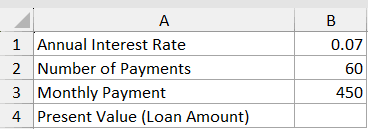
I want to figure out the present value, basically the loan amount that justifies $450 monthly payments at this rate for 5 years.
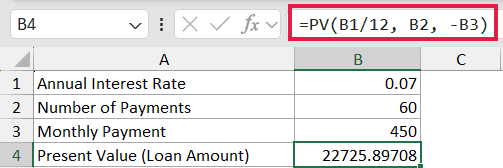
Here is the formula:
=PV(B1/12, B2, -B3)
How this formula works:
B1/12converts the annual interest rate (7%) into a monthly rate, because payments are monthly.B2is the number of monthly periods (60).-B3is the monthly payment ($450), entered as negative because it’s money going out of your pocket.
The result comes back as a positive number (around $22,727), which is the loan principal that $450 monthly payments would pay off over 60 months at 7% APR.
Pro Tip: If you ever see PV return a negative number when you expected positive (or vice versa), flip the sign on the PMT input. The sign convention is almost always the reason.
Example 2: Present Value of an Annuity
Here’s a scenario most retirement planning calculations involve.
Below is the dataset. A retirement plan will pay $2,000 per month for 20 years, and you want to know what that stream is worth today assuming a 5% annual discount rate.
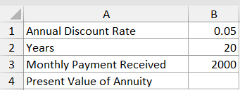
I want the lump-sum value of this annuity today, so I can compare it against a one-time cash offer.
Here is the formula:
=PV(B1/12, B2*12, B3)
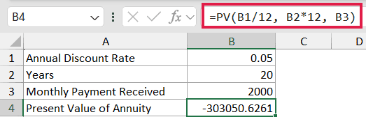
In the above formula, B1/12 converts the annual rate to monthly, B2*12 converts the 20 years into 240 months, and B3 is the $2,000 monthly inflow.
The result is negative (around -$303,000), which means you’d need to invest about $303,000 today to fund this annuity at 5%. If someone offers you a lump sum higher than that, the lump sum is the better deal.
Caveat: This example uses end-of-period payments (type defaulted to 0). If the annuity pays at the start of each month (an “annuity due”), add ,,1 at the end: =PV(B1/12, B2*12, B3, , 1). The present value will be slightly higher because each payment arrives one period earlier. If the annuity grows over time instead of staying flat, take a look at how to handle a growing annuity separately.
Example 3: Present Value of a Future Lump Sum
Now let’s look at a single future amount instead of a payment stream.
Below is the dataset. You’ll receive a $50,000 inheritance 8 years from now, and you want to know what that’s worth today at a 6% annual discount rate.
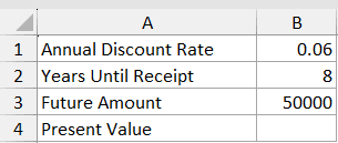
I want the present value of this single future amount, with no periodic payments involved.
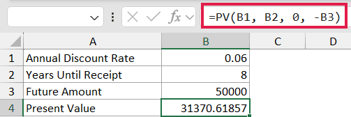
Here is the formula:
=PV(B1, B2, 0, -B3)
How this formula works:
B1is the annual rate (6%). Since there are no periodic payments, we keep everything in annual terms.B2is the number of years (8).0for the pmt argument, since no periodic payments are involved.-B3is the future value of $50,000, entered as negative because it’s an inflow you’ll receive later.
The result is around $31,370, which is what $50,000 received in 8 years is worth in today’s dollars.
This is mathematically the same as =50000/(1+0.06)^8, but PV handles it cleanly without writing out the discount formula manually. If you’re working in the other direction (figuring out what a present amount grows into over time), see the compound interest formula approach.
Example 4: Comparing Two Investment Offers
Here’s where PV really earns its keep.
Below is the dataset. Two investment offers are on the table. Offer A pays $1,200 monthly for 10 years. Offer B pays a single lump sum of $115,000 at the end of year 10. The discount rate is 5% annually.
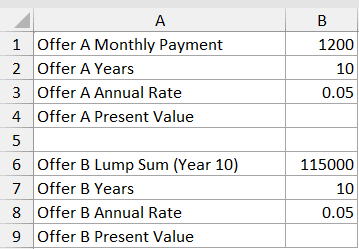
I want to compare both offers in today’s dollars so I can pick the better one.
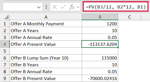
Here are the formulas:
=PV(0.05/12, 10*12, 1200)
=PV(0.05, 10, 0, 115000)
In the above formulas:
- The first one prices Offer A.
0.05/12is the monthly rate,10*12is 120 monthly periods, and1200is the monthly payment. - The second one prices Offer B. It’s a single future amount in 10 years, so pmt is 0 and the lump sum goes in as the fv argument.
Both results come back negative because they represent cash inflows from your perspective. Compare the absolute values. Whichever is larger in magnitude is worth more today.
Pro Tip: When comparing two streams, always discount them at the same rate and over the same time horizon. Mixing rates or periods makes the comparison meaningless. If you want to flip the question and ask “what return would make both offers equal?”, that’s where IRR comes in.
Example 5: PV with a Growing Set of Scenarios
Sometimes you want to evaluate several what-if scenarios at once instead of writing a separate formula for each one.
Below is the dataset. Each row shows a different rate, term, and monthly payment for a hypothetical loan, and you want the present value for every row.
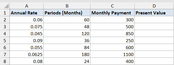
I want to fill the Present Value column for all rows in one go.
Here is the formula:
=PV(A2:A8/12, B2:B8, -C2:C8)
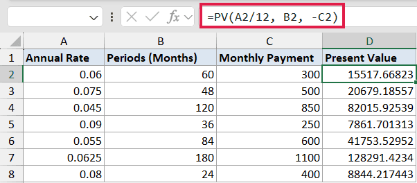
PV itself is a reducer (it returns a single value per call), but when you feed it arrays from three columns in Excel 365, it evaluates row by row and spills the results down column D. One formula fills all seven rows.
If you’re on Excel 2019 or older, this won’t spill. You’d need to enter =PV(A2/12, B2, -C2) in D2 and drag it down through D8 instead.
Caveat: This trick only works when every input column has the same number of rows. Mixing a 7-row range with a 5-row range will return a #N/A error past the shorter range.
Tips & Common Mistakes
- Mind the sign convention. Outflows are negative, inflows are positive. If your PV comes back with the wrong sign, flip the PMT or FV input.
- Match the rate to the period. Annual rate with monthly payments means dividing the rate by 12 AND multiplying the years by 12 in nper. Forgetting one of those is the most common PV mistake.
- PV is for constant payments only. If your cash flows vary period to period (one month $500, next month $700), use NPV instead with the actual cash flow series.
- The type argument matters more than people realize. A 20-year annuity paying at the start of each period (
type= 1) is worth noticeably more than one paying at the end. Check the structure before defaulting to 0. - Watch for negative interest rates. PV handles them mathematically, but the result can feel counterintuitive. Sanity check against a simpler calculation when rates are unusual.
- FV and PV are siblings. If you know any four of (rate, nper, pmt, pv, fv), you can solve for the fifth using the matching function. They all share the same sign convention.
PV is one of those functions that looks simple on the surface but quietly powers most of the financial calculations you’d ever do in Excel. The hardest part is remembering the sign convention. Once that clicks, loan pricing, annuity valuation, and offer comparisons all become one-line formulas.
Try it on a real decision you’re facing, like a mortgage you’re considering or a job offer with a deferred bonus. Seeing the present value next to the headline number often changes the picture.
Related Excel Functions / Articles: