
If you want to find a date before or after a set number of working days, the WORKDAY function is what you’re looking for.
In Excel 365, you can feed WORKDAY date and day ranges, and the results spill into the cells below. In this article, I’ll show you six practical ways to use it.
WORKDAY Function Syntax in Excel
The WORKDAY function returns a date before or after a starting date while skipping Saturdays, Sundays, and any holidays you supply.
=WORKDAY(start_date, days, [holidays])
start_dateis required. It is the date where Excel begins counting.daysis required. A positive number moves forward, while a negative number moves backward. Excel truncates a decimal value to an integer.[holidays]is optional. It is a range or array of dates that Excel must exclude from the working calendar.
WORKDAY returns an Excel date serial number. Format the result cell as a date to display it in a familiar form.
When to Use WORKDAY Function
- Calculate due dates that skip weekends
- Schedule work a set number of business days before a deadline
- Exclude company closures or public holidays from a timeline
- Move weekend and holiday dates to the next working day
- Find the last working day of a month
Example 1: Calculate Next Calibration Dates
Let’s begin with a schedule where every row has a different workday interval.
Below is a list of instruments with their last calibration dates and intervals in workdays. Column D will hold the next calibration dates.
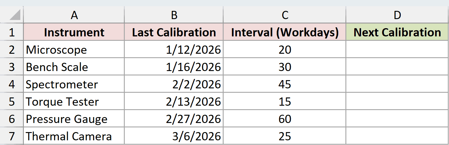
We want one formula to add each instrument’s interval while skipping Saturdays and Sundays.
Here is the formula:
=WORKDAY(B2:B7+0,C2:C7+0)
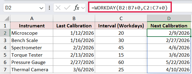
The first range supplies the six starting dates, and the second supplies the matching workday intervals. Adding zero leaves the values unchanged while making Excel evaluate both ranges as numeric arrays.
The results spill from D2 through D7. The Microscope’s next calibration is February 9, 2026, while the Bench Scale’s is February 27, 2026.
WORKDAY does not count the starting date as day one. It begins with the next working day when days is positive.
Example 2: Exclude Office Holidays
Now let’s see how the optional holidays argument changes a deadline.
Below is an application review table with submission dates and review periods. The office closure list is in G2:H4.

We first want the standard review dates with weekends excluded but office closures ignored.
Here is the standard formula:
=WORKDAY(B2:B6+0,C2:C6+0)
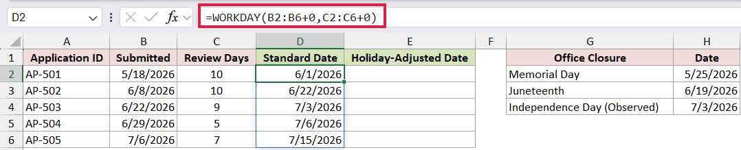
This formula uses only the required arguments. For AP-501, ten working days after May 18 is June 1, 2026.
Next, we want the same calculation to exclude the three dates in the closure list.
Here is the holiday-adjusted formula:
=WORKDAY(B2:B6+0,C2:C6+0,$H$2:$H$4)
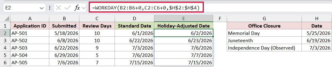
The absolute reference keeps the holiday range fixed. Memorial Day pushes AP-501 to June 2, and Juneteenth pushes AP-502 to June 23.
AP-505 stays at July 15 in both result columns because none of the listed closures falls inside its review period.
Pro Tip: Put actual Excel dates in the holiday range, not date-looking text. Microsoft notes that text dates can cause problems in WORKDAY formulas.
Example 3: Count Backward from an Opening Date
WORKDAY can schedule backward as easily as it schedules forward.
Below is a store-opening plan with one opening date, different lead times, and a closure list in F2:G4. Column D will show each task’s latest start date.
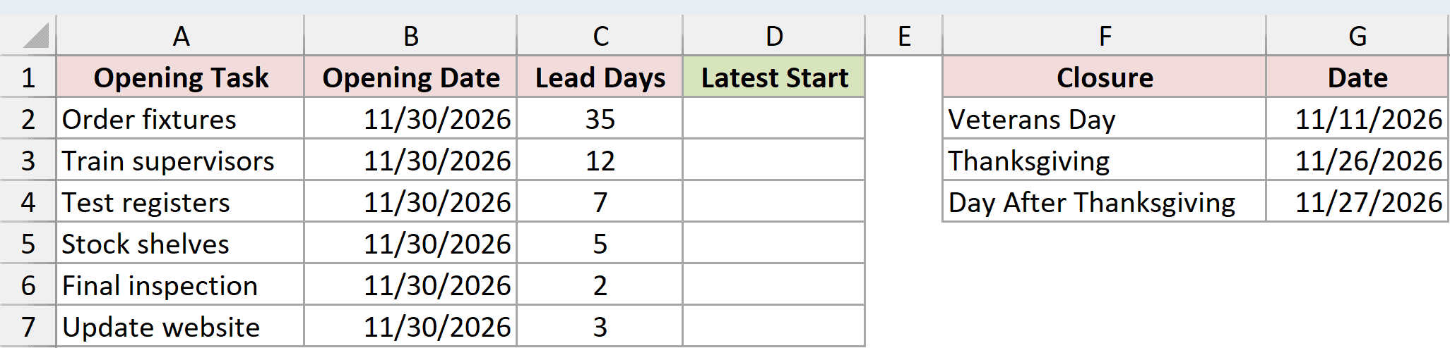
We want to subtract each lead time from the opening date while excluding weekends and closures.
Here is the formula:
=WORKDAY(B2:B7+0,-(C2:C7+0),$G$2:$G$4)
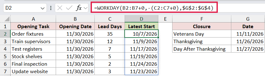
The minus sign changes each lead time to a negative offset, so WORKDAY moves into the past. The holiday range excludes Veterans Day, Thanksgiving, and the day after Thanksgiving.
Order fixtures must begin by October 7, 2026. Final inspection can begin on November 24 because it needs only two working days before the November 30 opening.
Example 4: Generate Available Workdays
Here’s a useful way to turn WORKDAY into a short availability list.
Below is a small scheduling card with a first available date, the number of slots, and two office closures. Column D will hold the available dates.
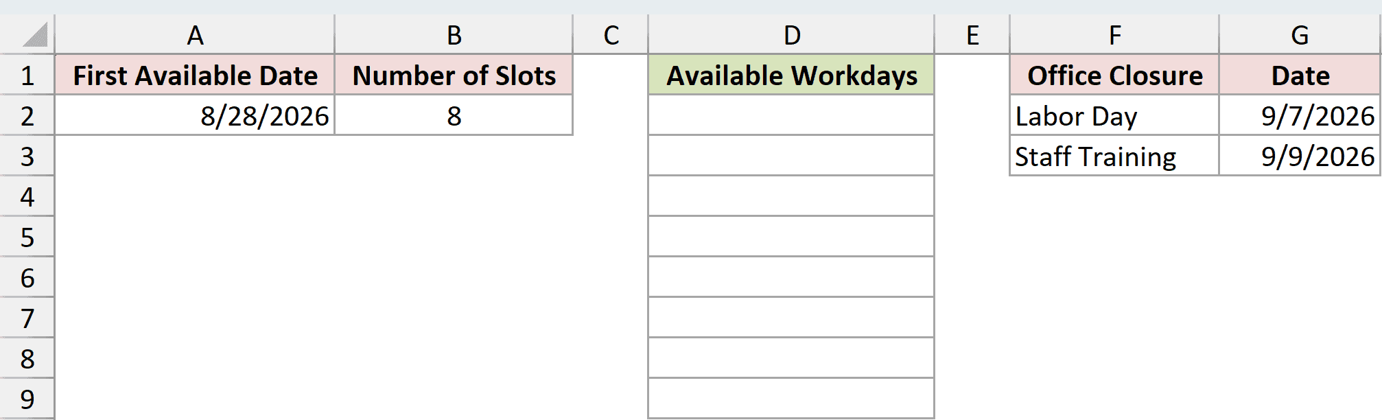
We want to generate the next eight working days while skipping the listed closures.
Here is the formula:
=WORKDAY(A2,SEQUENCE(B2),$G$2:$G$3)
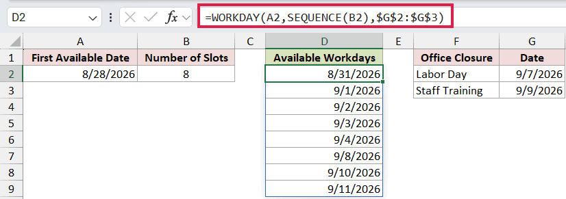
The SEQUENCE function returns the numbers 1 through 8. WORKDAY uses those numbers as offsets from August 28, so the result spills as eight dates.
The list starts on August 31. It skips the Labor Day closure on September 7 and the staff training closure on September 9.
This example requires Excel 2021, Excel 2024, or Microsoft 365 because SEQUENCE is not available in Excel 2019 or earlier.
Example 5: Move Payments to the Next Workday
This pattern is handy when a date may already be a valid working day.
Below is a payment-date list with two bank holidays in D2:E3. Column B will hold the adjusted dates.
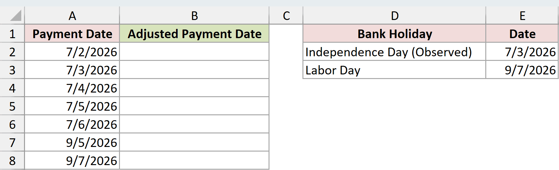
We want to keep valid working dates unchanged and roll weekends or holidays forward.
Here is the formula:
=WORKDAY(A2:A8-1,1,$E$2:$E$3)
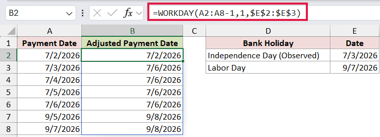
Subtracting one day and then adding one workday creates the roll-forward test. A valid workday returns to itself, while a weekend or holiday moves to the next available date.
July 2 stays July 2. July 3, July 4, and July 5 all move to July 6 because July 3 is in the holiday list and the next two days are a weekend.
The September dates show both rules together. September 5 is a Saturday, September 7 is Labor Day, and both move to September 8.
Example 6: Find the Last Workday of Each Month
For the last example, we’ll combine WORKDAY with a month-end calculation.
Below is a reporting-month list with two system-freeze dates in D2:E3. Column B will show the filing date for each month.
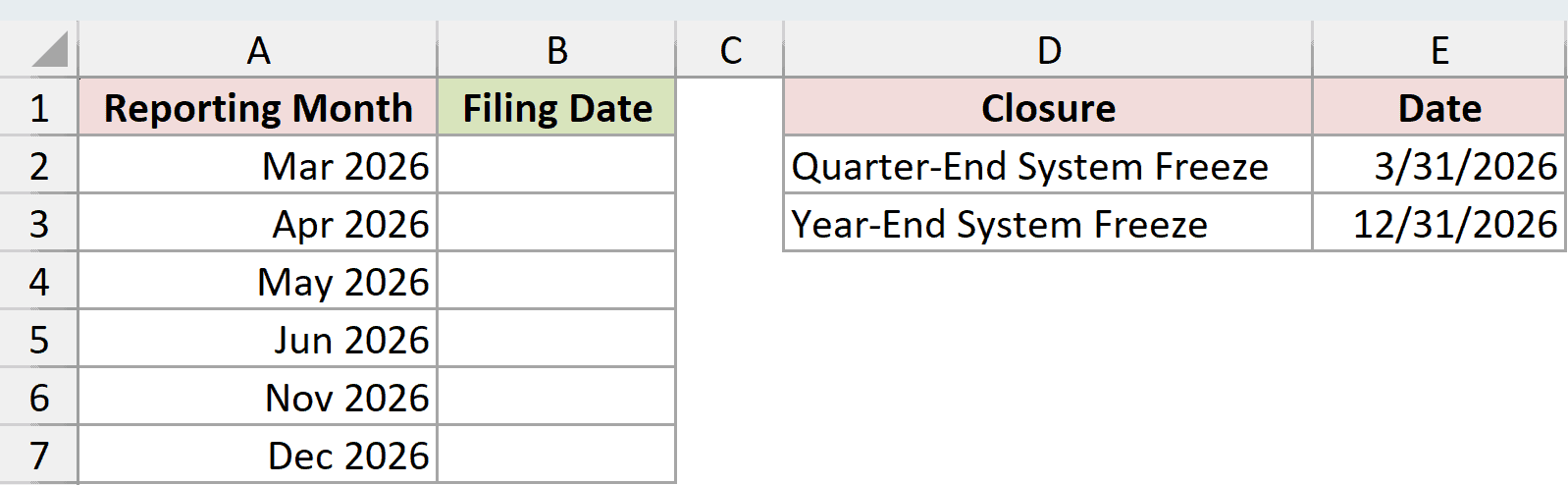
We want the last available workday of each month, with weekends and system freezes excluded.
Here is the formula:
=WORKDAY(EOMONTH(A2:A7+0,0)+1,-1,$E$2:$E$3)
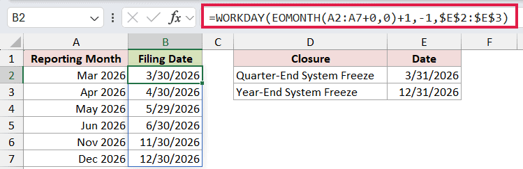
The EOMONTH function finds each calendar month-end, and adding one moves to the first day of the next month. WORKDAY then steps back one working day and skips any listed closure.
March 31 is a system freeze, so March’s filing date becomes March 30. May 31 falls on a Sunday, so May’s filing date becomes May 29.
December 31 is also a system freeze. The final filing date for that month is December 30.
Tips & Common Mistakes
- WORKDAY treats Saturday and Sunday as weekends. Use WORKDAY.INTL if your weekend falls on different days or lasts a different number of days.
- Use a positive
daysvalue for a future date and a negative value for a past date. - The start date is day zero. WORKDAY starts counting with the next or previous working day.
- If
dayscontains a decimal, WORKDAY truncates it rather than rounding it. - Holidays must be valid Excel dates. A holiday that already falls on a weekend does not remove an extra working day.
- WORKDAY returns a date. Use NETWORKDAYS when you need to count the working days between two dates.
- A spilled WORKDAY formula needs an empty result range. A blocked cell causes a
#SPILL!error.
I covered forward and backward scheduling, holiday exclusions, generated workday lists, payment adjustments, and month-end filing dates. I hope you found this article helpful.
Related Excel Functions / Articles:
