
If you want to find the compound growth rate between a starting value and an ending value, the RRI function gives you the rate for each period.
In this article, I’ll show you how to use RRI for investments, website traffic, declining values, savings goals, and input errors.
In Excel 365, you can also feed RRI ranges and the results will spill into the cells below.
RRI Function Syntax in Excel
The RRI function uses the number of periods, starting value, and ending value to calculate an equivalent growth rate per period.
=RRI(nper, pv, fv)
- nper (required) is the total number of compounding periods.
- pv (required) is the present value, or the value at the beginning of the first period.
- fv (required) is the future value, or the value at the end of the last period.
When to Use RRI Function
- Calculate the compound annual growth rate of an investment over several years.
- Find a monthly, quarterly, or annual growth rate from two values.
- Measure a compound rate of decline when the ending value is lower than the starting value.
- Work out the return needed to reach a future savings target.
- Compare RRI with the manual CAGR formula or the RATE function.
Example 1: Calculate Investment CAGR With RRI
Let’s start with a group of investments held for different lengths of time.
Below is the dataset. Columns B and C contain the invested and current values, while column D shows how many years each fund was held.
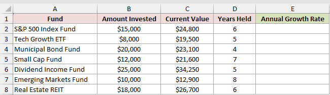
We want one formula to calculate the annual compound growth rate for every fund.
Here is the formula:
=RRI(D2:D8,B2:B8,C2:C8)
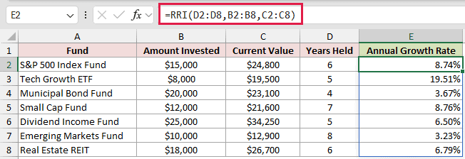
The years in column D become nper, the invested amounts in column B become pv, and the current values in column C become fv.
The formula spills seven results into E2:E8. The S&P 500 Index Fund returns 8.74%, while the Tech Growth ETF returns 19.51%.
Pro Tip: Keep E2:E8 empty before entering the formula. Any existing value in that output range will cause a #SPILL! error.
Example 2: Calculate Monthly and Annual Growth Rates
Now let’s measure website traffic growth over a full year.
Below is the dataset. Columns B and C show visits in January 2025 and January 2026, with two columns reserved for the calculated rates.
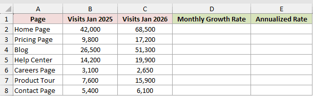
We want the monthly compound growth rate first, followed by its annualized equivalent.
Here is the monthly growth formula:
=RRI(12,B2:B8,C2:C8)
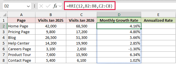
The first argument is 12, so RRI returns a monthly rate for the 12 monthly periods between the two values.
The Home Page grew by 4.16% per month. The Careers Page returns -1.30% because its visits fell during the year.
And here is the formula that converts each monthly rate into an annual rate:
=(1+D2:D8)^12-1
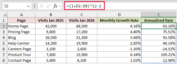
The formula adds 1 to each monthly rate, compounds it for 12 months, and subtracts 1. The Home Page annualized rate is 63.10%.
Because the starting and ending figures are exactly 12 months apart, this annualized rate also equals the total year-over-year change.
Pro Tip: RRI returns a rate per period. If nper counts months, the result is monthly. If it counts years, the result is annual.
Example 3: Calculate a Negative Growth Rate
Here’s what happens when some ending values are lower than their starting values.
Below is the dataset. It lists membership totals for seven gym locations in 2022 and 2026, with column D reserved for the annual change.
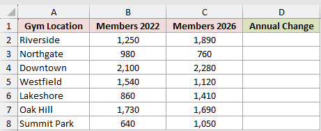
We want the annual compound change for each location across the four-year period.
Here is the formula:
=RRI(4,B2:B8,C2:C8)
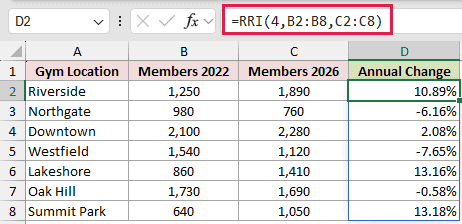
RRI needs no special adjustment for a decline. When the future value is smaller than the present value, the function returns a negative rate.
Northgate declined by 6.16% per year, and Westfield declined by 7.65%. Riverside grew by 10.89%, so its result remains positive.
Example 4: Compare RRI, CAGR, and RATE
Next, let’s calculate the same return three different ways.
Below is a parameter card with a starting value of $25,000, an ending value of $41,000, and a six-year holding period.

We want to confirm that RRI, the manual CAGR calculation, and RATE return the same result.
Here is the RRI formula:
=RRI(B3,B1,B2)
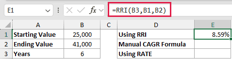
RRI takes the six years from B3, the starting value from B1, and the ending value from B2. It returns 8.59%.
And here is the manual CAGR formula:
=(B2/B1)^(1/B3)-1
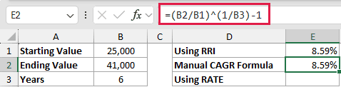
The manual formula divides the ending value by the starting value, takes the sixth root, and subtracts 1. It also returns 8.59%.
And here is the RATE formula:
=RATE(B3,0,-B1,B2)
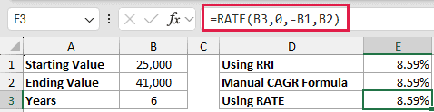
RATE uses six periods, zero recurring payments, a negative starting value, and a positive ending value. Its result is the same 8.59%.
The manual CAGR formula works in Excel versions that predate RRI. RATE is the better option when your calculation also includes recurring payments.
Pro Tip: RATE follows a cash-flow sign convention. Entering both B1 and B2 as positive values makes this formula return #NUM!, so the starting value uses -B1.
Example 5: Handle RRI #NUM! Errors
Finally, let’s calculate the return needed to reach several savings goals.
Below is the dataset. It contains the amount saved, target amount, and years remaining for seven goals, including two rows with invalid inputs.
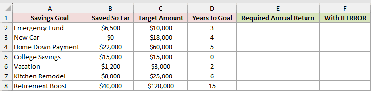
We want to calculate each required annual return and replace input errors with a readable message.
Here is the RRI formula:
=RRI(D2:D8,B2:B8,C2:C8)
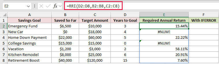
Most rows return a percentage. The Emergency Fund needs 15.44% per year, while the Home Down Payment needs 22.22%.
The New Car row returns #NUM! because its starting value is zero. College Savings returns the same error because its number of periods is zero.
Here is the formula that replaces those errors with a message:
=IFERROR(RRI(D2:D8,B2:B8,C2:C8),"Check inputs")
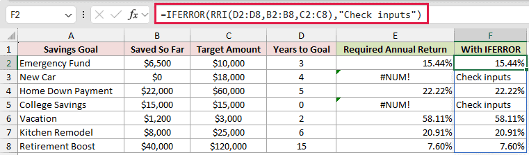
IFERROR keeps every valid percentage and displays “Check inputs” for the two invalid rows. That makes the spilled output easier to scan.
Pro Tip: nper must be greater than zero. pv and fv must be nonzero and share the same sign. RRI returns #VALUE! when an argument is nonnumeric.
Tips & Common Mistakes
- Match the unit in
nperto the rate you want. Twelve months returns a monthly rate, while five years returns an annual rate. - Format the result cells as percentages. A value such as 0.085944 represents 8.59%, not 0.09%.
- RRI is available in Excel 2013 and later. Use the manual CAGR formula when working in an older version.
- Leave the spill range empty in Excel 365. A blocked output cell causes a #SPILL! error.
- Use RATE instead when recurring deposits or withdrawals are part of the calculation.
- Check that
nperis greater than zero. Thepvandfvvalues must be nonzero numbers with the same sign.
RRI is a compact way to find the compound rate connecting two values across different time periods.
Related Excel Functions / Articles:
