
Excel’s RATE function returns the interest rate per period for an annuity with constant payments.
You can solve for a loan’s rate when you know its amount, payment, and term. The result uses the payment period, so monthly payments produce a monthly rate.
In this article, I’ll show you how to compare loan rates, convert monthly rates to annual rates, and estimate the return needed for a savings goal.
RATE Function Syntax in Excel
The RATE function uses the following syntax:
=RATE(nper, pmt, pv, [fv], [type], [guess])
nperis the required total number of payment periods.pmtis the required payment made each period. Use 0 when there are no periodic payments.pvis the required present value, or what the future payments are worth now.fvis the optional balance you want after the final payment. Excel uses 0 when you omit it.typeis optional. Use 0 or omit it for end-of-period payments, and use 1 for beginning-of-period payments.guessis an optional estimate of the rate. Excel uses 10% when you omit it.
When to Use RATE Function
- Find the interest rate implied by a loan amount, payment, and term.
- Calculate the return needed to reach a savings target.
- Compare plans with beginning-of-period and end-of-period payments.
- Solve for growth when there are no periodic payments.
Example 1: Compare Rates Across Loan Offers
Let’s start by comparing several financing offers.
Below is the dataset with the amount financed, term in years, and monthly payment for eight offers.
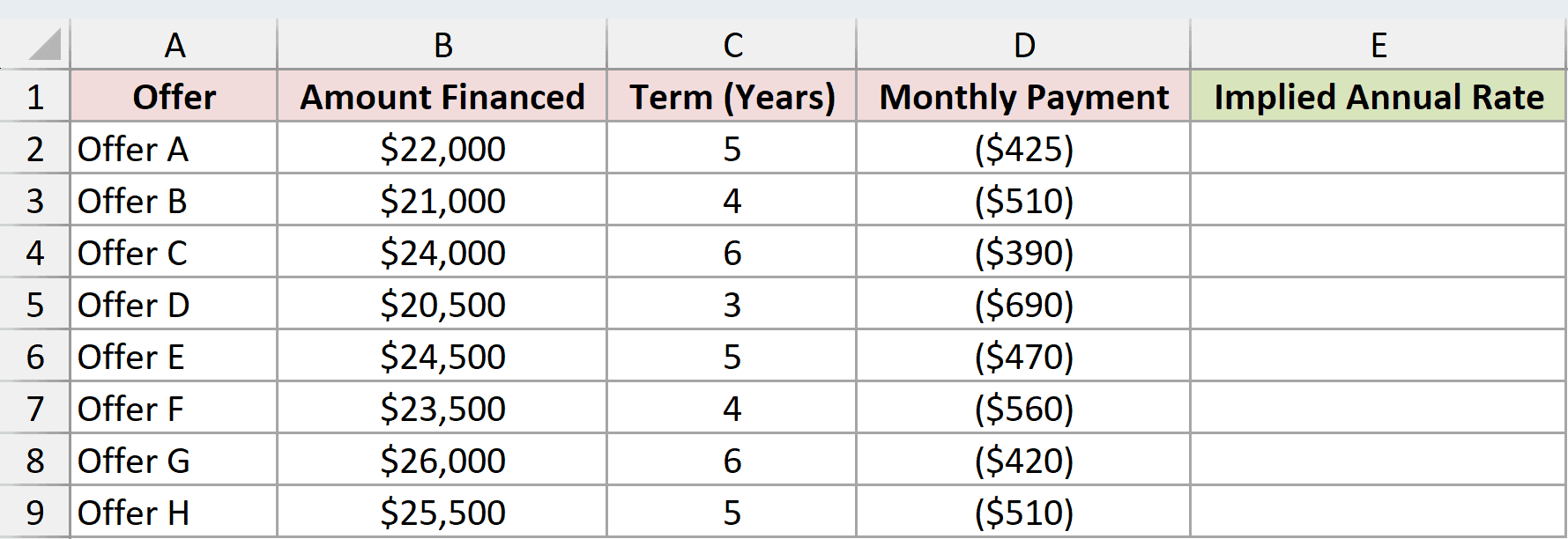
I want to calculate the implied nominal annual rate for every offer with one spilling formula.
Here is the formula:
=RATE(C2:C9*12,D2:D9,B2:B9)*12
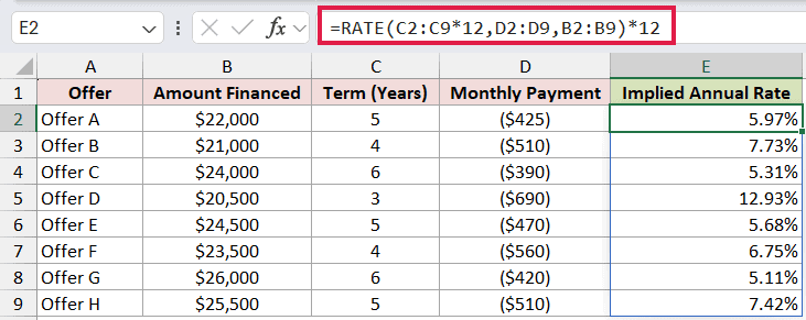
The terms in column C are years, so the formula multiplies them by 12 to get monthly periods. RATE returns a monthly rate, and the final *12 annualizes it.
The monthly payments are negative because they are cash paid out, while the financed amounts are positive. Offer G has the lowest implied annual rate at 5.11%, and Offer D has the highest at 12.93%.
The PMT function solves the opposite problem when you already know the rate and need the payment.
Example 2: Convert Monthly RATE to Annual Rates
A monthly rate can be annualized in two different ways.
Below is a loan with a $22,000 balance, a $425 monthly payment, and 60 payment periods.
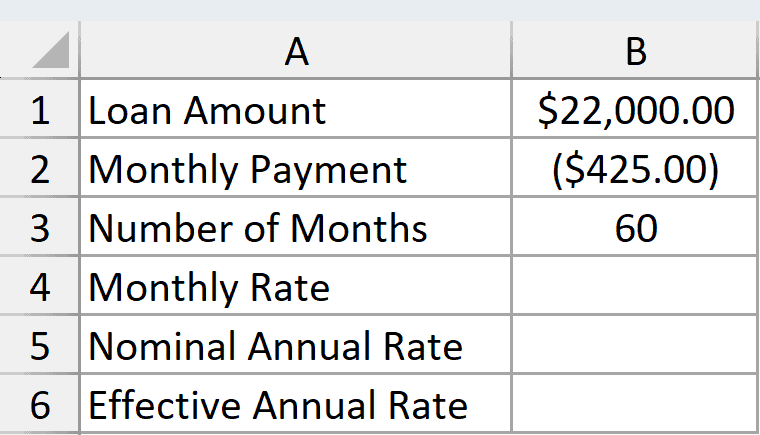
I want to compare the periodic rate, nominal annual rate, and effective annual rate for the same loan.
Here is the monthly rate formula:
=RATE(B3,B2,B1)
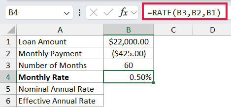
The monthly rate is 0.50% when displayed to two decimal places.
Here is the nominal annual rate formula:
=RATE(B3,B2,B1)*12
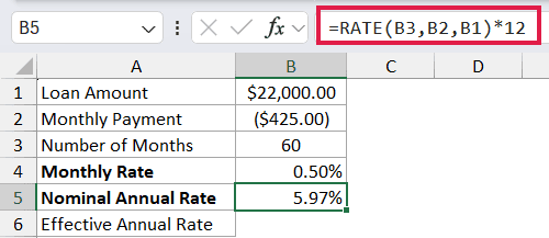
Multiplying by 12 gives a nominal annual rate of 5.97%.
Here is the effective annual rate formula:
=(1+RATE(B3,B2,B1))^12-1
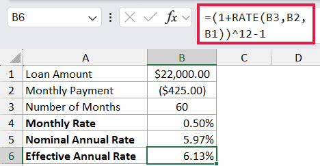
The effective rate is 6.13% because it includes monthly compounding. The EFFECT function can make this last conversion with =EFFECT(B5,12) once you have the nominal annual rate in B5.
RATE follows the same cash-flow sign convention used by the PV function. Money received and money paid must have opposite signs.
Example 3: Find a Required Savings Rate
RATE also works when the unknown is an investment return.
Below is the dataset with six savings plans, each with a starting balance, monthly deposit, time horizon, and target balance.
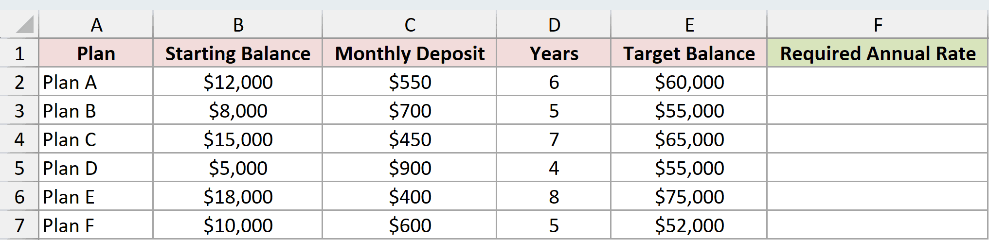
I want to calculate the nominal annual return each plan needs to reach its target.
Here is the formula:
=RATE(D2:D7*12,-C2:C7,-B2:B7,E2:E7,0)*12
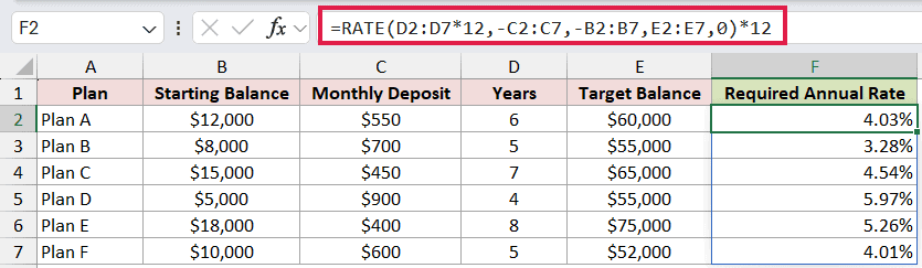
The formula converts years to monthly periods and treats the starting balance and deposits as cash paid into the plan. The target balance is cash received later, so it stays positive.
The required nominal annual rates run from 3.28% for Plan B to 5.97% for Plan D.
If the deposits happen on irregular dates, the XIRR function is more appropriate because it uses the actual cash-flow dates.
Example 4: Compare Deposit Timing With RATE
The type argument tells RATE when each payment happens.
Below is a savings goal with a $10,000 starting balance, $500 monthly deposits, a 60-month term, and a $50,000 target.
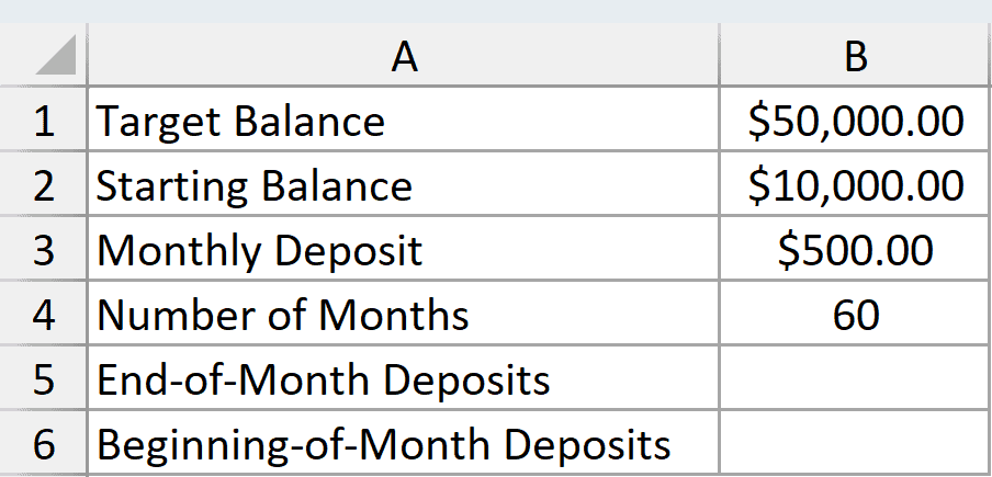
I want to compare the required rates when deposits occur at the end and beginning of each month.
Here is the formula for end-of-month deposits:
=RATE(B4,-B3,-B2,B1,0)*12
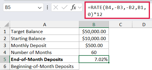
With type set to 0, the required nominal annual rate is 7.02%.
Here is the formula for beginning-of-month deposits:
=RATE(B4,-B3,-B2,B1,1)*12
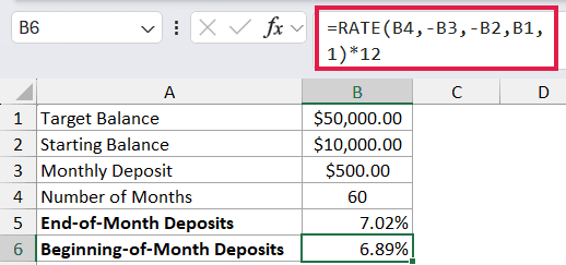
With type set to 1, the required rate falls to 6.89%. Each deposit has one extra month to earn a return, so the plan does not need quite as high a rate.
Pro Tip: Use 0 for payments at the end of each period and 1 for payments at the beginning. If you omit type, Excel uses 0.
Example 5: Estimate a Rate With a Buyout
The optional fv and guess arguments help with financing that leaves a final balance.
Below is an equipment plan with a $36,000 price, $900 monthly payments, 48 months, and a $4,000 end-of-term buyout.
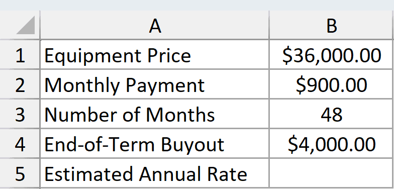
I want to estimate the nominal annual rate implied by the payments and final buyout.
Here is the formula:
=RATE(B3,-B2,B1,-B4,0,1%)*12
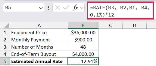
The equipment price is positive because it represents value received. The monthly payments and buyout are negative because they are paid out.
The FV function uses the same future-value argument and sign convention. Here, -B4 tells RATE that $4,000 remains payable after the monthly payments.
The 1% guess gives Excel’s iterative calculation a monthly starting point. RATE converges on a nominal annual result of 12.91%.
Example 6: Calculate Growth Without Payments
RATE can calculate growth even when there are no recurring cash flows.
Below is a reserve that grows from $18,000 to $30,000 over seven years.
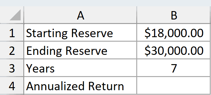
I want to calculate the annual return that connects the starting and ending balances.
Here is the formula:
=RATE(B3,0,-B1,B2)
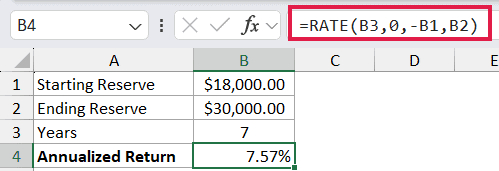
There are seven annual periods, and the payment argument is 0. The starting reserve is negative and the ending reserve is positive, so RATE returns an annual growth rate of 7.57%.
When you have only a starting value, ending value, and period count, RRI is shorter: =RRI(B3,B1,B2). RATE also handles recurring payments and payment timing.
Tips & Common Mistakes
- RATE returns a rate per period. Keep
nper,pmt, andguesson the same monthly, quarterly, or annual basis. - Cash paid and cash received must have opposite signs. If every cash flow has the same sign, RATE cannot solve the equation.
- RATE uses iteration. If it does not converge after 20 iterations, Excel returns
#NUM!; changingguesscan help. - A nominal annual rate from monthly periods uses
*12. An effective annual rate must also account for compounding. - Microsoft lists RATE for Excel 2016 and later.
- In Excel 365, a range-based RATE formula spills automatically. A blocked output range returns
#SPILL!, while implicit intersection reduces the formula to one result. - In older Excel versions without dynamic arrays, use a row-level RATE formula and copy it down.
I’ve shown you how RATE solves for loan rates, savings returns, payment timing, final buyouts, and growth without payments. I hope you found this article helpful.
Related Excel Functions / Articles:
