REGEXEXTRACT Function in Excel

If you want to pull numbers, email addresses, or other patterned text from messy cells, the REGEXEXTRACT function can save a lot of manual cleanup.

It is available only in Excel for Microsoft 365 on Windows and Mac.

You’ll see how to write patterns that find the text you need and control what REGEXEXTRACT returns.

REGEXEXTRACT is a dynamic array function that spills its results across the cells below or beside the formula.

REGEXEXTRACT Function Syntax in Excel

The REGEXEXTRACT function searches text for a regular expression pattern and returns the matching text.

=REGEXEXTRACT(text, pattern, [return_mode], [case_sensitivity])

• text (required) is the text or cell reference you want to search.
• pattern (required) is the regular expression that describes the text you want to extract.
• return_mode (optional) controls the result. Use 0 or omit it for the first match, 1 for every match, or 2 for capture groups from the first match.
• case_sensitivity (optional) controls letter case. Use 0 or omit it for case-sensitive matching, or use 1 for case-insensitive matching.

When to Use REGEXEXTRACT Function

• Pull numbers, codes, email addresses, or phone numbers from longer text strings.
• Return every occurrence of a pattern when one cell contains several matching values.
• Split structured text into separate columns by using capture groups.
• Match text regardless of capitalization by changing the case sensitivity setting.
• Extract values whose position varies from one cell to another.

Example 1: Extract First Number from Product Text

Let’s start with product listings that contain pack sizes in different positions.

Below is the dataset. Column A contains eight product descriptions with a first number to extract from each listing.

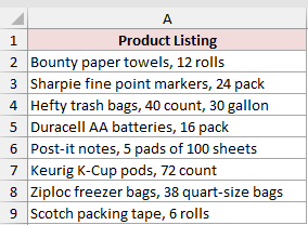
We want to extract the first run of digits from every description, first as text and then as a number.

Here is the formula that returns text:

=REGEXEXTRACT(A2:A9,"\d+")

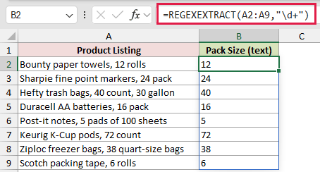
And here is the formula that converts each result into a number:

=VALUE(REGEXEXTRACT(A2:A9,"\d+"))

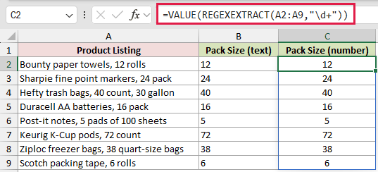
The pattern \d+ means one or more digits. REGEXEXTRACT finds the first matching run in each cell and spills all eight results down column B.

REGEXEXTRACT always returns text, even when the match contains only digits. VALUE converts those results into real numbers in column C, ready for calculations.

For example, the first listing returns 12, and the Post-it listing returns 5 rather than the later 100.

Pro Tip: REGEXEXTRACT returns the first match by default. Use return_mode 1 when you need every match in a cell.

Example 2: Extract an Email Address from Text

A common cleanup job is finding email addresses buried inside notes.

Below is the dataset. Column A contains seven free-form support notes, each with an email address buried in the text.

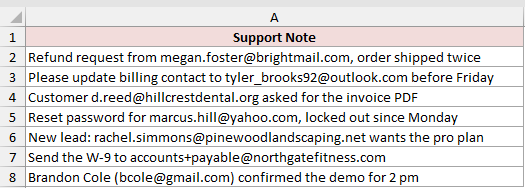
We want one spilling formula to pull the email address from all seven notes.

Here is the formula:

=REGEXEXTRACT(A2:A8,"[A-Za-z0-9._%+-]+@[A-Za-z0-9.-]+\.[A-Za-z]{2,}")

The first character class matches the mailbox name. It allows letters, numbers, and common symbols such as periods, underscores, percent signs, plus signs, and hyphens.

The @ matches itself, while the next character class matches the domain. \. finds the literal period before the final two or more letters.

The address can appear anywhere in the note. Its position does not need to be consistent from one row to the next.

Example 3: Extract Phone Numbers and Handle No Match

Phone numbers get trickier when some rows don’t contain one.

Below is the dataset. Column A contains eight contact notes, including two with no phone number in the expected format.

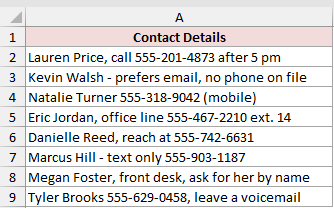
We want column B to return each phone number or the message “No phone found”.

Here is the formula:

=IFERROR(REGEXEXTRACT(A2:A9,"\d{3}-\d{3}-\d{4}"),"No phone found")

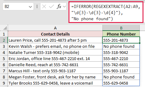
Each \d{3} section matches exactly three digits, and \d{4} matches four. The hyphens in the pattern match the hyphens in each phone number.

REGEXEXTRACT returns #N/A when it finds no match. IFERROR replaces that error for Kevin Walsh and Megan Foster with a clearer message.

This pattern finds a number anywhere in the text, but it requires the exact 555-201-4873 format shown here.

Pro Tip: Adjust the pattern if your phone data includes parentheses, spaces, country codes, or inconsistent separators. A fixed pattern only matches the format it describes.

Example 4: Return Every Match with return_mode 1

Let’s move to cells that can contain more than one matching value.

Below is the dataset. Column A contains seven customer messages, each with one to three order IDs in the text.

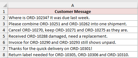
We want each row to return every order ID mentioned in its customer message.

Enter this formula in B2 and copy it down through B8:

=REGEXEXTRACT(A2,"ORD-\d{5}",1)

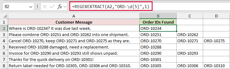
ORD- matches the fixed prefix, while \d{5} matches the five digits that follow it. The final 1 tells REGEXEXTRACT to return every match.

Each row’s formula spills horizontally. A message with one order ID fills only column B, while a message with three IDs fills columns B through D.

This example uses a copied formula because each source row needs its own horizontal spill range.

To keep all matches in one cell, you can wrap the formula in TEXTJOIN, such as =TEXTJOIN(", ",TRUE,REGEXEXTRACT(A2,"ORD-\d{5}",1)).

Example 5: Extract Capture Groups from an Address

Capture groups can split the final parts of a US address into separate columns.

Below is the dataset. Column A contains eight full addresses with a city, state, and ZIP code.

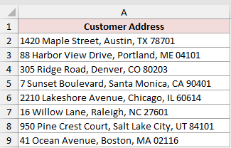
We want one formula on each row to extract the three address parts into neighboring cells.

Enter this formula in B2 and copy it down through B9:

=REGEXEXTRACT(A2,", ([A-Za-z ]+), ([A-Z]{2}) (\d{5})$",2)

The three parenthesized sections are capture groups. They match the city, the two-letter state code, and the five-digit ZIP code.

The leading comma and space prevent the city result from starting with an extra space. The $ anchors the match to the end of the address.

The final 2 returns the three capture groups as a horizontal array. In row 2, the formula spills Austin, TX, and 78701 across columns B through D.

Because REGEXEXTRACT returns text, ZIP codes such as 04101 and 02116 keep their leading zeros.

Example 6: Make Regex Matching Case Insensitive

Finally, let’s compare case-sensitive and case-insensitive matching.

Below is the dataset. Column A contains seven ticket subjects, including Dashboard chart takes forever, medium priority.

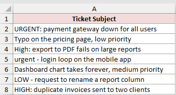
We want to see which priorities the default formula misses, then make the matching ignore capitalization.

Here is the default case-sensitive formula:

=REGEXEXTRACT(A2:A8,"urgent|high|medium|low")

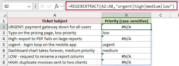
To show how the final argument changes the result, here is the case-insensitive formula:

=REGEXEXTRACT(A2:A8,"urgent|high|medium|low",0,1)

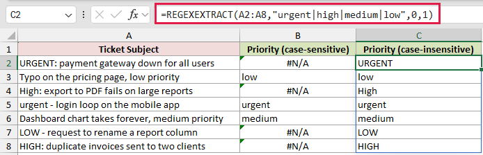
The pipe character means “or,” so the pattern can match any of the four priority words.

The first formula uses the default case-sensitive setting. It returns #N/A for URGENT, High, LOW, and HIGH because their capitalization does not match the pattern.

In the second formula, 0 keeps the default first-match return mode. The final 1 makes the search case-insensitive, so every row returns a priority.

The dashboard ticket returns medium in both columns.

Tips & Common Mistakes

• REGEXEXTRACT is available only in Excel for Microsoft 365 on Windows and Mac. Other current and perpetual Excel versions may return #NAME?.
• REGEXEXTRACT always returns text. Wrap it in VALUE when you need to calculate with extracted digits.
• A missing match returns #N/A. Use IFERROR when a missing value is expected and you want a friendlier result.
• return_mode 2 returns capture groups from the first match only. You cannot combine all-match behavior with capture-group output in the same REGEXEXTRACT call.
• REGEXEXTRACT uses PCRE2 regular expressions. Small pattern changes can alter what matches, so test a new pattern against several realistic rows.
• Spilled results need empty cells. If anything blocks the output area, Excel returns #SPILL!.
• Return mode 1 and return mode 2 can spill across columns. Leave enough empty cells to the right of each formula.

Patterns such as \d+ and ORD-\d{5} keep the formula focused on the text you actually want.

Start with the first-match default, then use return modes 1 and 2 when you need every match or separate capture groups.

List of All Excel Functions

Related Excel Functions / Articles:

• SEARCH Function in Excel
• TEXTAFTER Function in Excel
• How to Check If a Cell Contains Text in Excel?