
If you want to return a set number of rows or columns from an edge of a range, TAKE is built for the job.
TAKE is a dynamic array function. It spills the rows or columns you asked for into the cells below and to the right.
In this article, I’ll show you how to take blocks from the top, bottom, left, and right of your data.
TAKE is available in Microsoft 365 and Excel 2024. Excel 2021 and earlier return a #NAME? error.
TAKE Function Syntax in Excel
The TAKE function returns a contiguous block from the start or end of an array.
=TAKE(array, rows, [columns])
- array (required) is the range or array containing the data you want to return.
- rows (required for row selection, but skippable when columns is supplied) specifies how many rows to return. A positive number takes rows from the top, while a negative number takes them from the bottom.
- columns (optional) specifies how many columns to return. A positive number takes columns from the left, while a negative number takes them from the right.
Excel also accepts a skipped rows argument when columns is supplied, even though Microsoft’s argument table labels rows as required.
When to Use TAKE Function
- Return the first or last few records from a list.
- Keep a set number of columns from either edge of a wide table.
- Extract a rectangular block from one corner of a range.
- Return the highest or lowest records after sorting a list.
- Keep one part of an array while DROP returns the remaining part.
Example 1: Take the First Five Rows
Let’s start with the most common TAKE setup.
Below is the dataset. Columns A through D contain 12 freight shipments with destinations, dates, and weights.
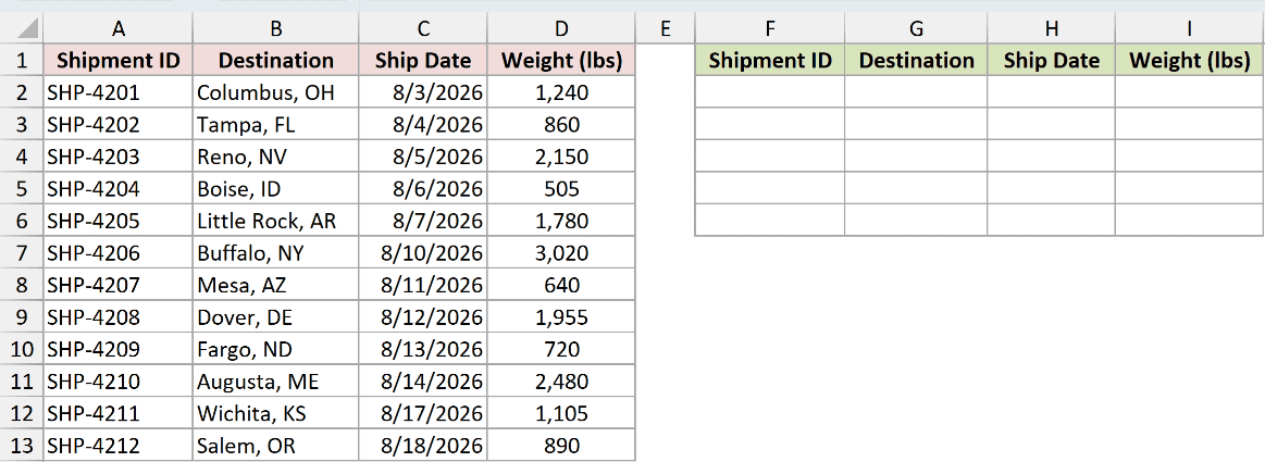
We want to return the first five shipment records from A2:D13.
Here is the formula:
=TAKE(A2:D13,5)
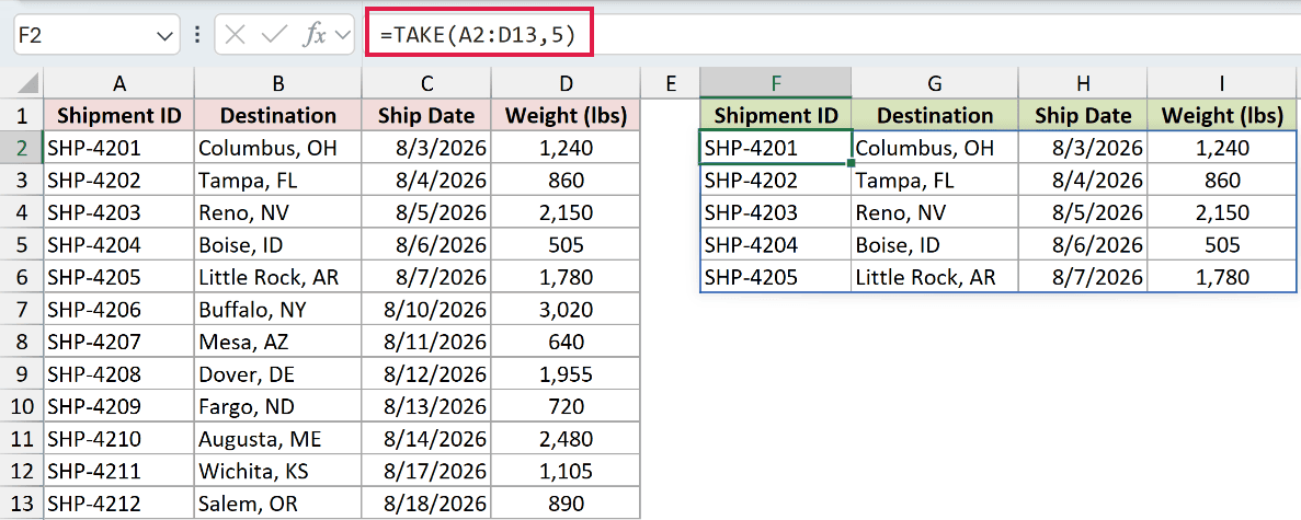
The positive row count tells TAKE to start at the top. The formula spills five rows and all four columns into F2:I6.
The result starts with SHP-4201 for Columbus and ends with SHP-4205 for Little Rock. I typed the result headers in row 1 separately.
Pro Tip: If the array includes the header row, =TAKE(A1:D13,6) returns that header as the spill’s first row. The count is 6 because it includes one header and five data rows.
Example 2: Take the Last Three Rows
Now let’s take records from the other end of a list.
Below is the dataset. Columns A through D hold a donation log arranged by receipt date from earliest to latest.
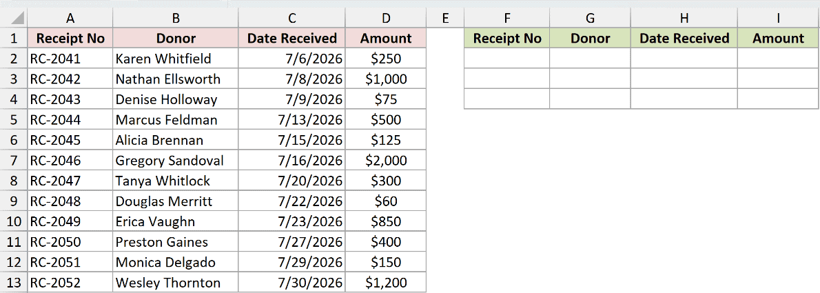
We want to return the final three receipts in the date-ordered log.
Here is the formula:
=TAKE(A2:D13,-3)
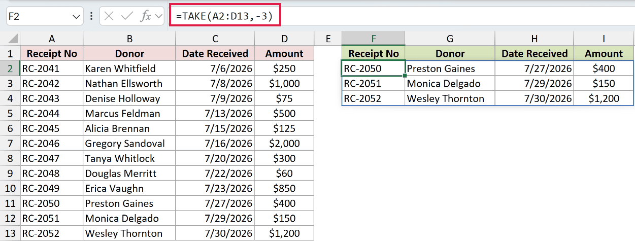
The negative row count makes TAKE work upward from the bottom. It returns receipt numbers RC-2050, RC-2051, and RC-2052.
Those receipts were received on July 27, July 29, and July 30, with amounts of $400, $150, and $1,200.
TAKE is positional, so these are the latest receipts only because the source is already sorted by date.
Example 3: Take Columns From Either Edge
Here’s how to use TAKE across columns instead of rows.
Below is the dataset. Columns A through F contain ten HVAC work orders with customer, service, technician, hours, and billing details.
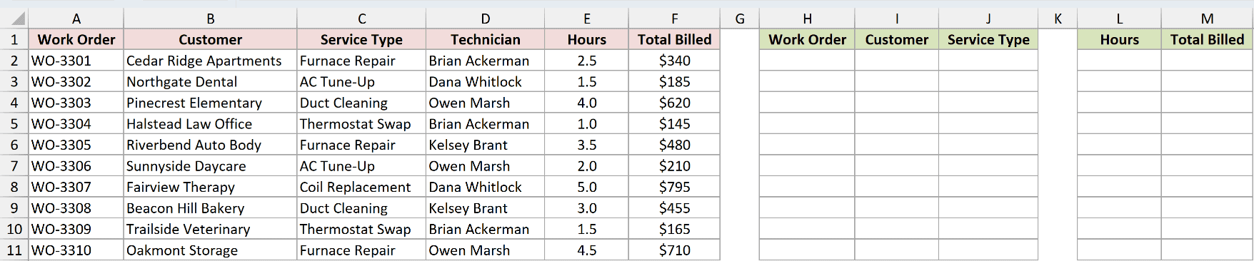
We want every work order row, first with the leftmost three columns and then with the rightmost two columns.
Here is the formula for the first three columns:
=TAKE(A2:F11,,3)
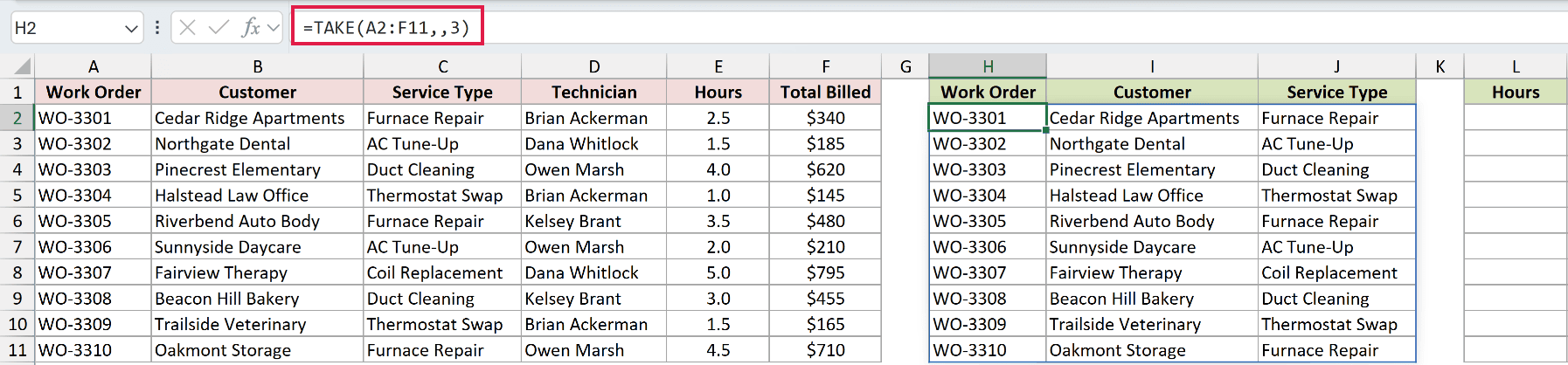
The double comma skips the rows argument, so TAKE keeps every row. The positive 3 returns data from the Work Order, Customer, and Service Type columns, not their labels.
Here is the formula for the last two columns:
=TAKE(A2:F11,,-2)
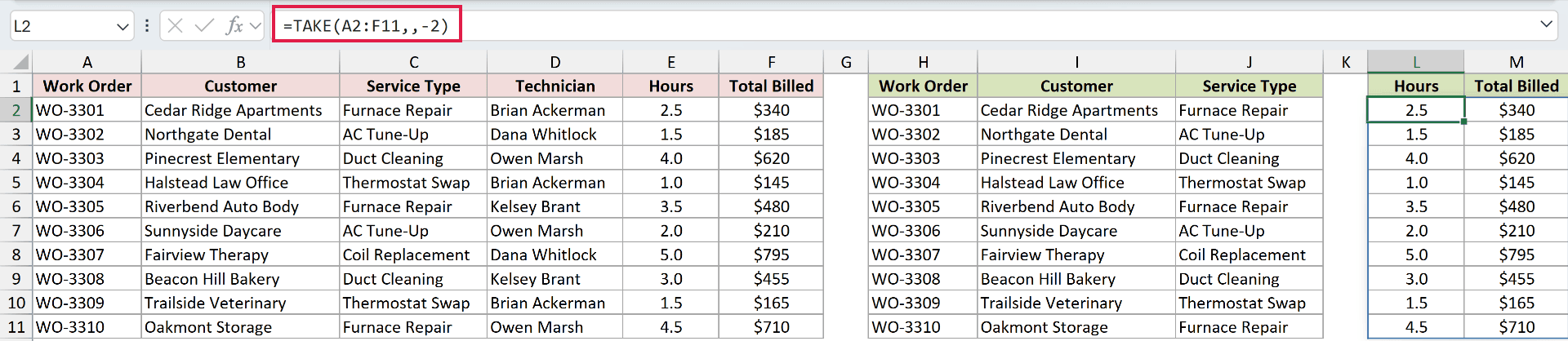
The skipped rows argument still keeps every record. This time, the negative 2 returns data from the Hours and Total Billed columns, not their labels.
For example, WO-3301 returns 2.5 hours and $340, while WO-3310 returns 4.5 hours and $710.
CHOOSECOLS is useful when the columns aren’t next to each other or don’t start at an edge. TAKE is shorter for a contiguous edge block.
Example 4: Take a Corner Block
Let’s use row and column counts together.
Below is the dataset. Columns A through E list 12 volunteer entries with events, dates, hours, and miles driven.
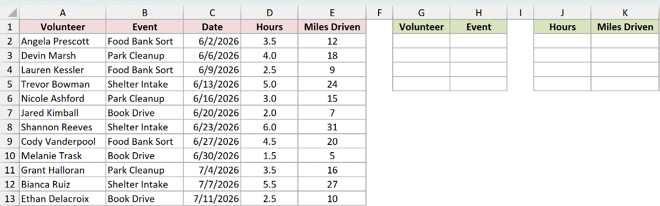
We want the top-left four-by-two block and the bottom-right four-by-two block from the same range.
Here is the formula for the top-left block:
=TAKE(A2:E13,4,2)
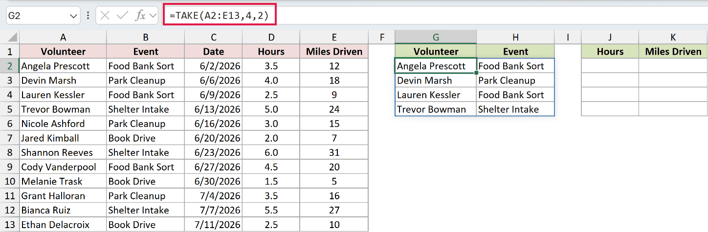
Both counts are positive, so TAKE starts at the top and left. The result contains the first four volunteers and their events.
Here is the formula for the bottom-right block:
=TAKE(A2:E13,-4,-2)
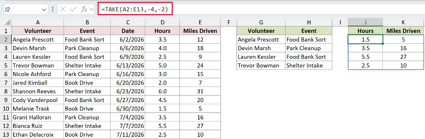
Both counts are negative, so TAKE starts at the bottom and right. The result contains Hours and Miles Driven for the last four entries.
The first row of that block has 1.5 hours and 5 miles. The last row has 2.5 hours and 10 miles. The signs control the edge, not the displayed order.
Example 5: Get Top Records With TAKE
Now let’s put TAKE after sorting and filtering.
Below is the dataset. Columns A through C contain 15 podcast episodes with categories and download counts.
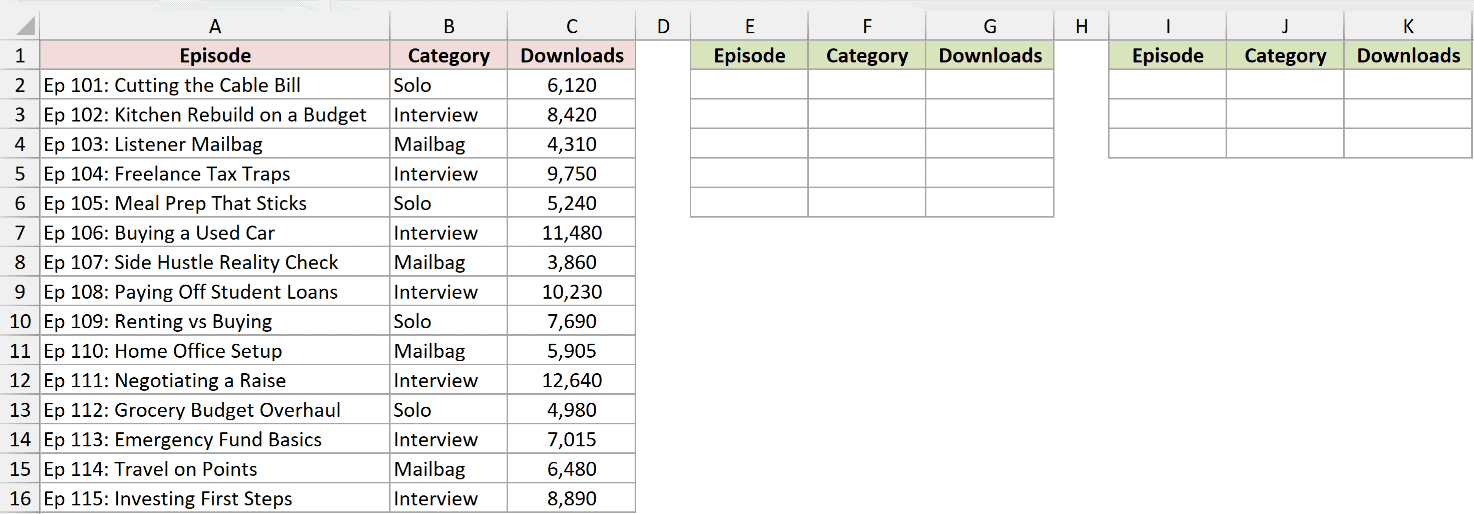
We want the five most-downloaded episodes overall, followed by the three most-downloaded Mailbag episodes.
Here is the formula for the overall top five:
=TAKE(SORT(A2:C16,3,-1),5)
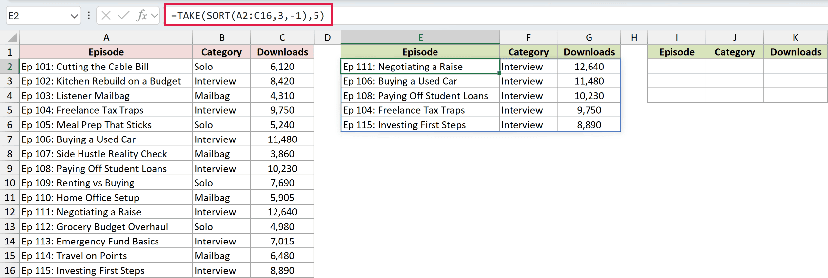
SORT arranges the rows by the third column in descending order. TAKE then keeps the first five rows from that sorted array.
The result runs from Negotiating a Raise with 12,640 downloads to Investing First Steps with 8,890 downloads.
Here is the formula for the top three Mailbag episodes:
=TAKE(SORT(FILTER(A2:C16,B2:B16="Mailbag"),3,-1),3)
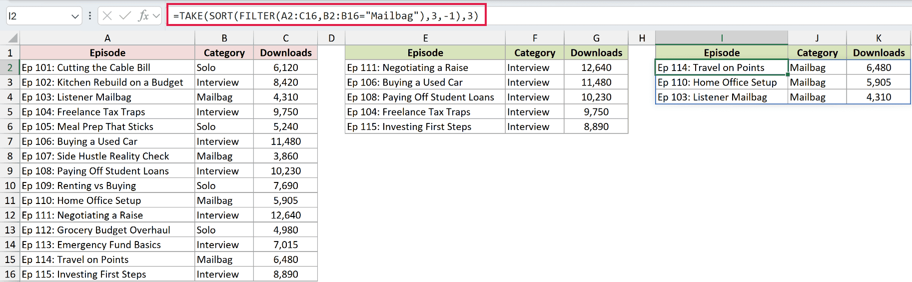
FILTER first keeps only Mailbag rows. SORT orders those rows by downloads, and TAKE returns the first three.
The result is Travel on Points with 6,480 downloads, Home Office Setup with 5,905, and Listener Mailbag with 4,310.
SORTBY can be easier than SORT when the sort key sits outside the columns you want to return.
Example 6: TAKE vs DROP
Finally, let’s compare TAKE with its closest companion.
Below is the dataset. Columns A through C contain 12 newsletter sends with send dates, subject lines, and open counts.
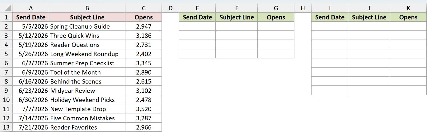
We want TAKE to keep the first four sends and DROP to return everything after those four.
Here is the TAKE formula:
=TAKE(A2:C13,4)
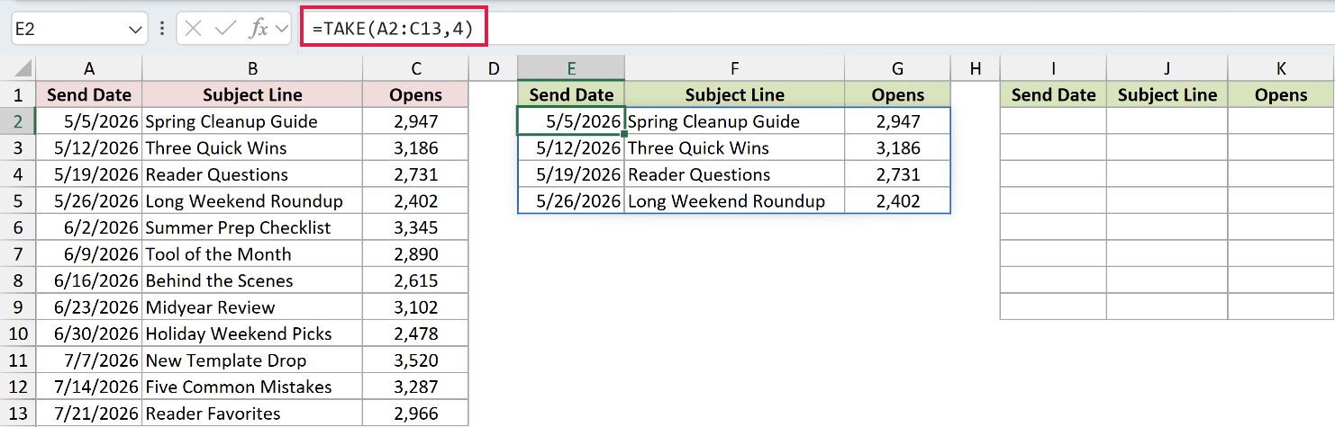
TAKE keeps the first four rows, from Spring Cleanup Guide through Long Weekend Roundup.
Here is the DROP formula:
=DROP(A2:C13,4)
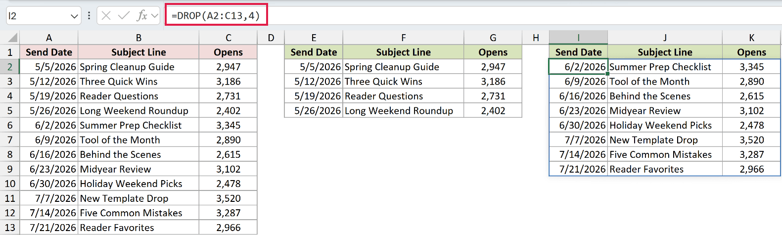
DROP removes those same four rows and returns the remaining eight. Its result starts with Summer Prep Checklist and ends with Reader Favorites.
TAKE keeps the specified edge block, and DROP removes it.
Tips & Common Mistakes
- TAKE counts positions, not logical records. Blank rows inside the source still count, and trailing blanks can appear in a result. Use a Table or FILTER to clean the source first.
- A row or column count of 0 returns #CALC! because TAKE would have to return an empty array.
- Asking for more rows or columns than the array contains doesn’t cause an error. TAKE returns the maximum available size, so you do not need to cap a row request with MIN and ROWS.
- Keep the spill area empty. A blocked output cell causes #SPILL! because Excel cannot place the full result.
- You can use a spilled range as the source. For example,
=TAKE(E2#,5)takes five rows from the array beginning at E2. - To extract a middle section, nest the functions.
=TAKE(DROP(A2:C13,3),4)skips three rows and returns the next four. - LARGE returns top values, but it does not preserve their matching rows as TAKE does after SORT arranges the full dataset.
- TAKE always returns a contiguous block from an edge. Use CHOOSEROWS or CHOOSECOLS when you need non-adjacent positions.
TAKE gives you a compact way to keep a block from any edge of an array.
Sort the source first when “first” or “last” needs to follow a date, score, or another value.
Related Excel Functions / Articles:
Other Excel articles you may also like:
