
Excel’s SORTBY function sorts an array using values from one or more corresponding arrays.
You can order a report by a column that is not included in the output. Multiple sort keys let you sort within categories and break ties.
In this article, I’ll show you how to sort by multiple columns, apply a custom priority order, and sort a filtered list.
SORTBY Function Syntax in Excel
The SORTBY function returns a sorted copy of a range or array based on one or more matching sort arrays.
=SORTBY(array, by_array1, [sort_order1], [by_array2, sort_order2], ...)
arrayis required. It is the range or array you want Excel to return in sorted order.by_array1is required. It supplies the first row or column of values to sort by.[sort_order1]is optional. Use1for ascending order or-1for descending order. Excel uses ascending order if you omit it.[by_array2, sort_order2]is an optional additional sort pair. You can add more pairs when you need more sorting levels.
Each sort array must line up with the rows or columns in array. SORTBY is available in Excel 2021, Excel 2024, and Microsoft 365.
When to Use SORTBY Function
- Create a sorted view without rearranging the source table
- Sort by a column that does not appear in the returned result
- Apply two or more sorting levels in one formula
- Arrange labels in a custom business order
- Filter rows and sort the remaining records with one formula
Example 1: Sort Appointments by Date
Let’s start with a simple ascending sort.
Below is a service schedule with IDs, customers, appointment dates, and service types. Columns F through I will hold the sorted copy.
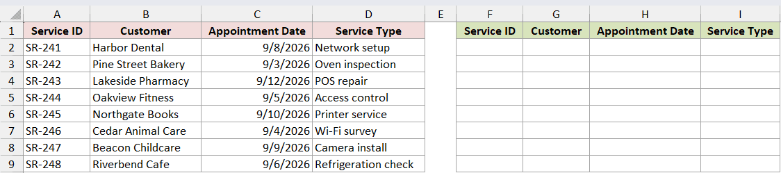
We want to sort every service row by the appointment date in column C.
Here is the formula:
=SORTBY(A2:D9,C2:C9,1)
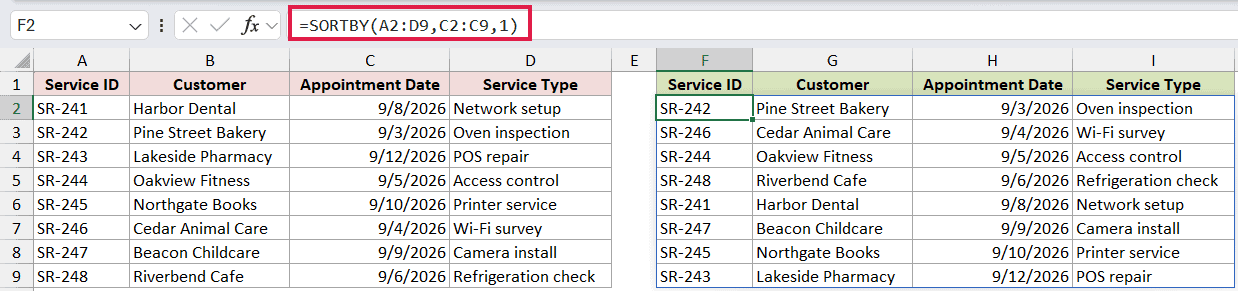
The array is A2:D9, so all four columns stay together. C2:C9 supplies the sort values, and 1 puts the dates in ascending order.
Pine Street Bakery’s September 3 appointment appears first. Lakeside Pharmacy’s September 12 appointment appears last.
Because the sort column is inside the returned array, the SORT function can also handle this example with =SORT(A2:D9,3,1). SORTBY becomes more useful when the sort key sits outside the returned columns.
Example 2: Sort by a Column Not Returned
A separate sort key is useful when the output should stay compact.
Below is a production-lot table with lot details and a rework rate in column D. The output in columns F through H leaves the rate out.
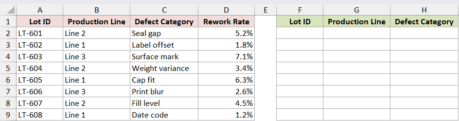
We want to return the first three columns while sorting the lots by rework rate from highest to lowest.
Here is the formula:
=SORTBY(A2:C9,D2:D9,-1)
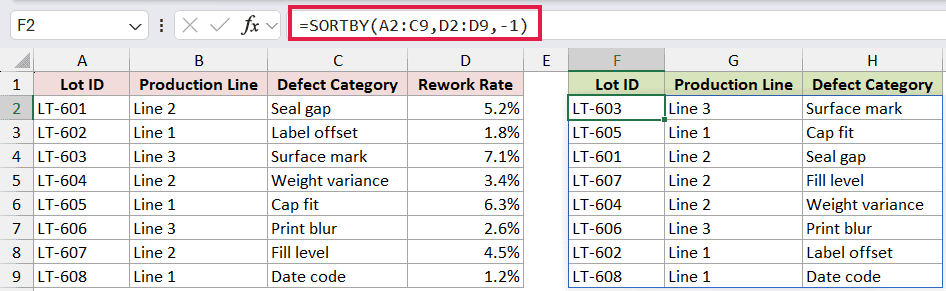
A2:C9 controls what the formula returns, while D2:D9 supplies a separate sort key. The -1 argument applies descending order.
Lot LT-603, with the highest rework rate of 7.1%, appears first. LT-608, with the lowest rate of 1.2%, appears last.
Pro Tip: The sort range and return range do not need the same number of columns. They only need the same number of rows when you are sorting rows.
Example 3: Sort by Multiple Columns
SORTBY can break ties with another sort level.
Below is a laboratory sample log with a test category, received date and time, and status. Columns F through I will hold the sorted result.
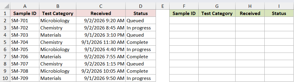
We want to group the samples by test category, then place the earliest received sample first within each group.
Here is the formula:
=SORTBY(A2:D10,B2:B10,1,C2:C10,1)
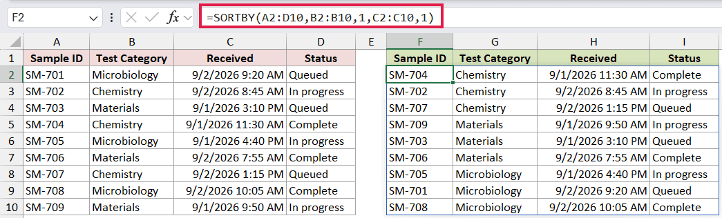
The first pair, B2:B10 and 1, sorts the categories alphabetically. The second pair, C2:C10 and 1, sorts the received times from earliest to latest inside each category.
The Chemistry group comes first. Within that group, SM-704 appears before SM-702 and SM-707 because it has the earliest received time.
SORTBY evaluates the sort pairs from left to right. Put the main grouping key first and the tie-breaking key second.
Example 4: Sort in a Custom Priority Order
Alphabetical order does not always match the order a business needs.
Below is a maintenance-request list and a custom urgency order in E2:E4. Columns G through I will hold the prioritized requests.
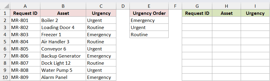
We want Emergency requests first, followed by Urgent requests and then Routine requests.
Here is the formula:
=SORTBY(A2:C10,XMATCH(C2:C10,E2:E4),1)
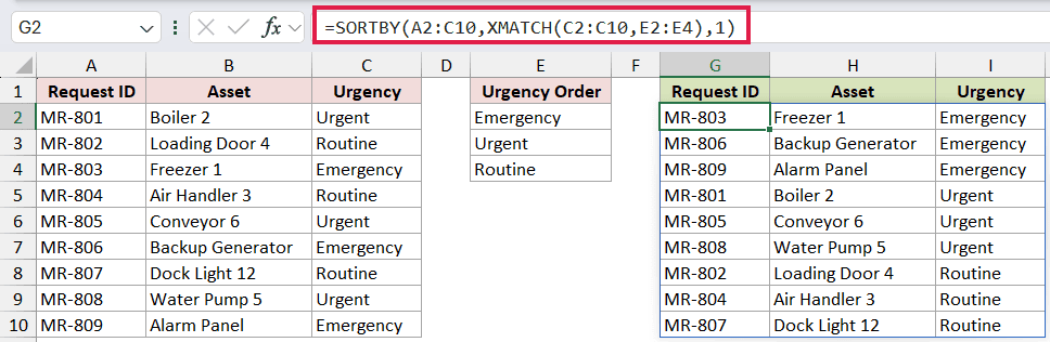
The XMATCH function compares every urgency label in C2:C10 with the list in E2:E4. It returns position 1 for Emergency, 2 for Urgent, and 3 for Routine.
SORTBY uses those positions as its sort values. The three emergency requests rise to the top, and the routine requests move to the bottom.
If you change the order in E2:E4, the spilled result updates to follow the new priority.
Example 5: Sort Dates by Month and Day
Sometimes the year should not affect the order.
Below is an asset register with installation dates from several years. Columns E through G will hold an anniversary list sorted through the calendar year.
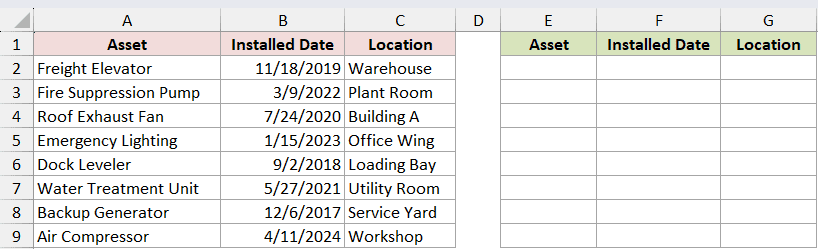
We want to sort the assets by installation month and day while ignoring the installation year.
Here is the formula:
=SORTBY(A2:C9,TEXT(B2:B9,"mmdd"),1)
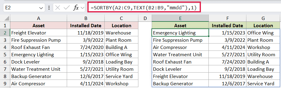
The TEXT function converts each date to a four-digit month-and-day key. For example, January 15 becomes 0115, while November 18 becomes 1118.
SORTBY arranges those keys in ascending order. Emergency Lighting appears first with a January 15 anniversary, and Backup Generator appears last with a December 6 anniversary.
You can also use separate MONTH and DAY sort arrays. The TEXT version keeps the same logic in one compact sort key.
Example 6: Filter First, Then Sort
Here, the support queue only needs its open cases.
Below is a support-case table with case type, age in days, and status. Columns F through H will show open cases from oldest to newest.
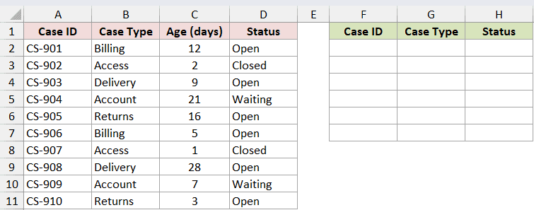
We want to filter out closed and waiting cases, hide the age column, and sort the remaining open cases by age.
Here is the formula:
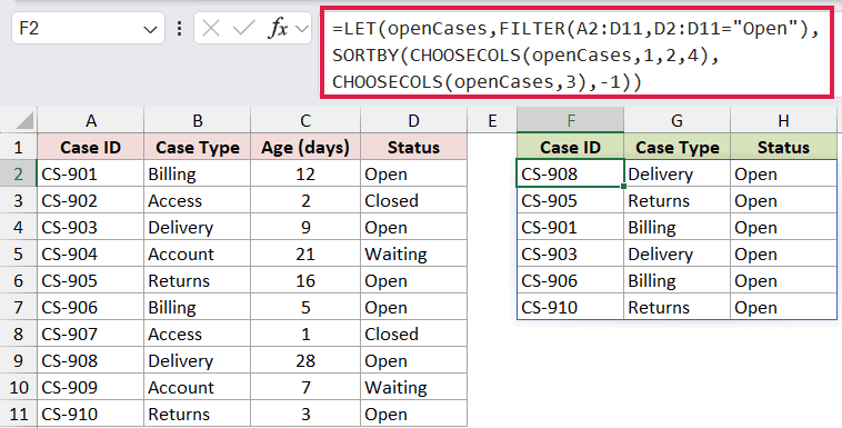
=LET(openCases,FILTER(A2:D11,D2:D11="Open"),SORTBY(CHOOSECOLS(openCases,1,2,4),CHOOSECOLS(openCases,3),-1))
How this formula works:
- The FILTER function keeps only the rows where the status in D2:D11 is Open.
- LET assigns the filtered four-column array to the name
openCases. - The first CHOOSECOLS returns the case ID, case type, and status columns.
- The second CHOOSECOLS returns the age column as the sort key.
- SORTBY uses
-1to place the oldest open case first.
The result starts with CS-908 at 28 days and ends with CS-910 at 3 days. The age values control the order but do not appear in the returned array.
Pro Tip: This example requires Microsoft 365 or Excel 2024 because CHOOSECOLS is not available in Excel 2021. The first five examples work in Excel 2021.
Tips & Common Mistakes
- SORTBY uses ascending order when you omit a sort-order argument. Enter
-1when you need descending order. - Every
by_arraymust match the height or width of the array being sorted. Mismatched dimensions return an error. - Keep the spill area empty. Any value blocking the output range causes a
#SPILL!error. - You cannot edit one cell inside a spilled result. Change the source data or the formula at the spill anchor instead.
- If the source is an Excel table, put the SORTBY formula outside the table. Structured references let the result resize as the source table changes.
- Use a spill reference such as
F2#when another formula needs the entire SORTBY result. - SORTBY creates a separate sorted view. Use Excel’s Sort command when you want to rearrange the source rows themselves.
I covered single-key, hidden-key, multilevel, custom-order, anniversary, and filter-then-sort formulas. I hope you found this article helpful.
Related Excel Functions / Articles:
Other Excel articles you may also like:
