
If you want to count how many columns a range contains, the COLUMNS function gives you that number without doing the count yourself.
In this article, I’ll show you how to use COLUMNS for range sizes, flexible lookups, last-column calculations, and split text.
COLUMNS returns a single number, but it also works inside dynamic array formulas such as =COLUMNS(TEXTSPLIT(A2,", ")).
COLUMNS Function Syntax in Excel
The COLUMNS function takes one array or reference and returns its number of columns.
=COLUMNS(array)
- array (required) is a continuous cell range, an array constant, or an array returned by another formula.
In an array constant such as {1,2,3;4,5,6}, commas separate columns and semicolons separate rows. That constant has three columns, so COLUMNS returns 3.
When to Use COLUMNS Function
- Count the fields in a dataset or report.
- Calculate the total cells in a rectangular range when combined with ROWS.
- Create a flexible VLOOKUP column index that adjusts when a column is inserted.
- Point INDEX to the final column of a fixed range without counting its position.
- Count items after TEXTSPLIT separates text across columns.
Example 1: Count Columns in a Range
Let’s start with the most direct use of COLUMNS.
Below is the dataset. It lists nine inventory items across six fields: item code, item, category, unit price, on-hand quantity, and reorder level.
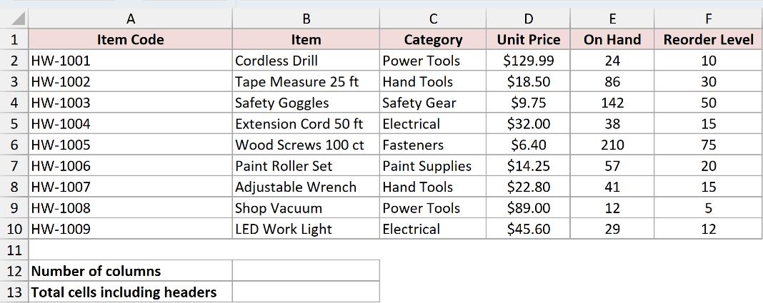
We want to find the table’s width in columns.
Here is the formula:
=COLUMNS(A1:F10)
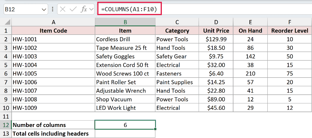
The range runs from column A through column F, so the formula returns 6.
Now let’s count every cell in the same range, including the header row.
Here is the formula:
=COLUMNS(A1:F10)*ROWS(A1:F10)
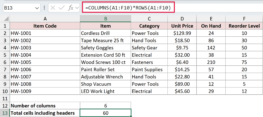
COLUMNS returns 6 and ROWS returns 10. Multiplying them gives 60 cells.
The number of rows never changes the COLUMNS result. For example, a one-row range and a hundred-row range can both be two columns wide.
Example 2: COLUMNS vs COLUMN
This distinction is easy to mix up, so let’s put both functions beside the same table.
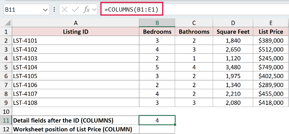
Below is the dataset. It contains eight property listings with bedrooms, bathrooms, square feet, and list price after the listing ID.
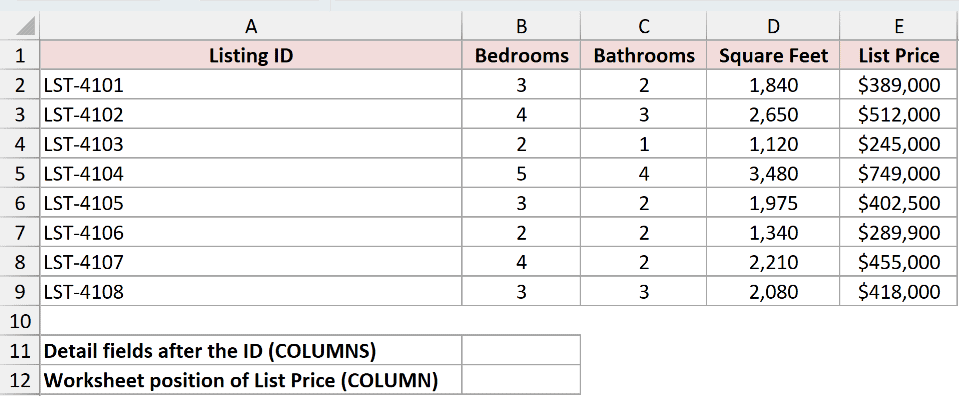
We want to compare how many detail fields the table has with the worksheet position of List Price.
Here is the COLUMNS formula:
=COLUMNS(B1:E1)
And here is the COLUMN formula:
=COLUMN(E1)
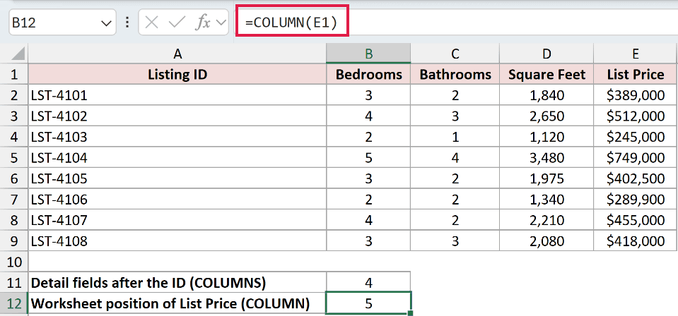
COLUMNS returns 4 because B, C, D, and E make four columns. COLUMN returns 5 because E is the worksheet’s fifth column.
COLUMNS answers “how many?” while COLUMN answers “which worksheet position?”
Example 3: Flexible VLOOKUP Column Index
Here’s a practical way to make an older VLOOKUP formula less fragile.
Below is the dataset. It shows an employee directory and a lookup card containing the employee ID EMP-2075.
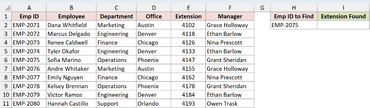
We want to return that employee’s extension without hard-coding VLOOKUP’s column index as 5.
Here is the formula:
=VLOOKUP(H2,$A$2:$F$11,COLUMNS($A$1:$E$1),FALSE)
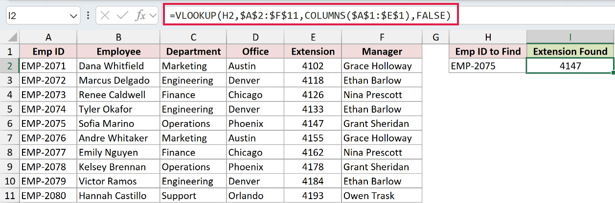
COLUMNS counts five fields from A through E, so VLOOKUP returns the fifth field in its table. For EMP-2075, that extension is 4147.
If someone inserts a column inside columns A through E, Excel widens both references. COLUMNS then supplies the adjusted index, keeping the formula pointed at Extension.
In Excel 2021, Excel 2024, and Microsoft 365, =XLOOKUP(H2,$A$2:$A$11,$E$2:$E$11) does the same job without a column index. The VLOOKUP pattern still helps in older workbooks.
Example 4: Get the Last Column With COLUMNS
Now let’s use COLUMNS to point INDEX at the end of a range.
Below is the dataset. It shows revenue for eight branches from January through June.
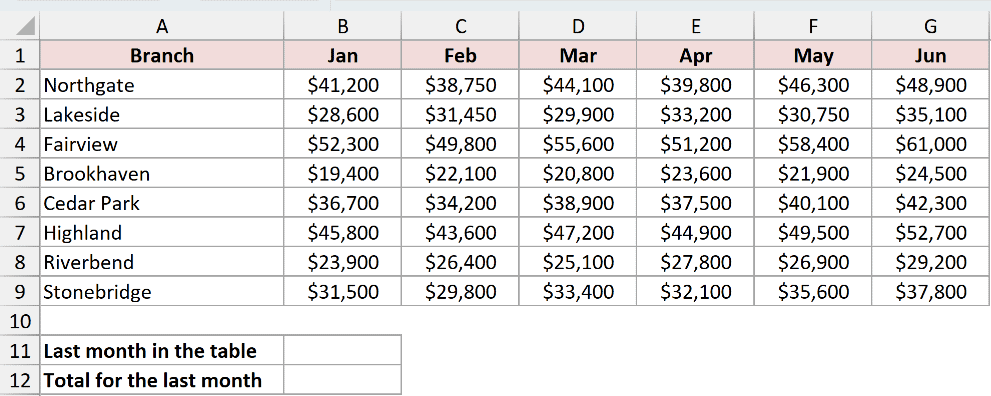
We want to identify the last month in the range and total its revenue without manually counting the month columns.
First, use this formula to return the last month label:
=INDEX(B1:G1,COLUMNS(B1:G1))
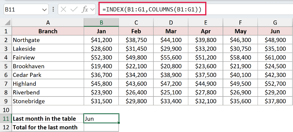
The range B1:G1 contains six columns, so COLUMNS gives INDEX a column number of 6. INDEX returns Jun.
Next, use this formula to total the final revenue column:
=SUM(INDEX(B2:G9,0,COLUMNS(B2:G9)))
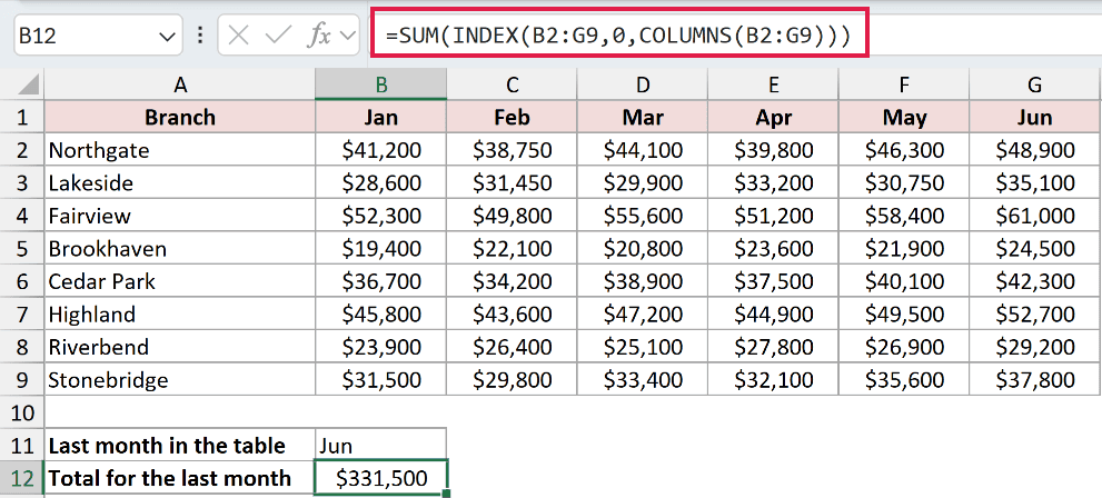
The zero tells INDEX to return every row from the sixth column. SUM then adds those June values and returns $331,500.
This removes the hand-counted column number. It also survives a column inserted inside the range because Excel adjusts the reference.
It does not automatically include a new month added outside B:G. In Excel 2024 and Microsoft 365, TAKE can pull the final column more directly with =TAKE(B1:G1,,-1).
Example 5: Count Comma-Separated Items
Finally, let’s count items stored together in one cell.
Below is the dataset. It contains order IDs and comma-separated item lists for eight hardware orders.
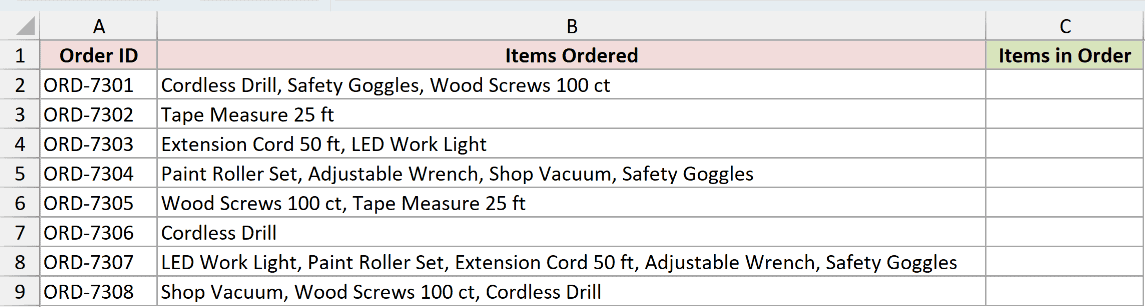
We want to count how many items appear in each order.
Enter this formula in C2, then copy it down through C9:
=COLUMNS(TEXTSPLIT(B2,", "))
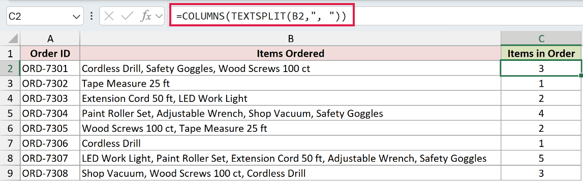
TEXTSPLIT separates each list into columns at each comma-plus-space pair. COLUMNS then counts the resulting columns and returns one number for that row.
The copied formulas return 3, 1, 2, 4, 2, 1, 5, and 3 for the eight orders.
TEXTSPLIT requires Excel 2024 or Microsoft 365. In older versions, =LEN(B2)-LEN(SUBSTITUTE(B2,",",""))+1 counts the commas and adds one.
Tips & Common Mistakes
- COLUMNS counts width, not cells. If the range has many rows, combine COLUMNS with ROWS as shown in Example 1.
- COLUMNS needs one continuous range. A multi-area reference such as
(A1:B2,D1:E2)returns#REF!, so give COLUMNS one continuous range. =COLUMNS(Table1)counts an Excel Table’s current width. The structured reference expands when you add a Table column, making this a self-extending option.=COLUMNS(A:D)returns 4. By contrast,=COLUMNS(1:1)returns 16,384 because a full worksheet row spans every Excel column.- COLUMN reports worksheet position, so the first field of a table starting in column D has position 4. COLUMNS is not affected by where the range starts.
=COLUMNS($A$1:A1)creates a 1, 2, 3 counter when copied across. In Excel 2021, Excel 2024, and Microsoft 365, SEQUENCE is usually clearer for creating that row of numbers.- COLUMNS can count the width of a spilled range. For example,
=COLUMNS(E2#)returns the spill’s current column count and works well inside other dynamic array formulas.
COLUMNS is most useful when a formula needs a range’s width instead of a hard-coded position.
Revisit Example 3 for a flexible VLOOKUP index, or Example 4 when you need the last column in a fixed range.
Related Excel Functions / Articles:
