If you want to find out which row a cell sits in, or generate a running list of numbers without typing them by hand, the ROW function is what you reach for. It returns the row number of a reference, or of the cell holding the formula itself.
That sounds simple, but ROW quietly powers a lot of useful tricks, from auto-numbering lists to flagging every other row. In Excel 365, you can also feed ROW a range and the row numbers spill into the cells below.
ROW Function Syntax in Excel
The ROW function takes a single optional argument.
=ROW([reference])
- reference (optional) – the cell or range you want the row number of. Leave it out and ROW returns the row number of the cell the formula is in.
When to Use ROW Function
- Auto-number a list so the numbers update when you add or delete rows.
- Build a dynamic index inside INDEX, OFFSET, or LARGE so each row pulls the next item.
- Flag every other row (or every Nth row) for banded shading and conditional formatting.
- Read off the row position of a specific cell when troubleshooting a formula.
- Create a spilled 1..N sequence in a single formula in Excel 365.
Example 1: Get the Current Row Number
Let’s start with the simplest case.
Below is a short staff list with names in column A and departments in column B.
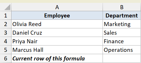
We want to know the row number of the cell that holds the formula, so we use ROW with no argument.
Here is the formula:
=ROW()
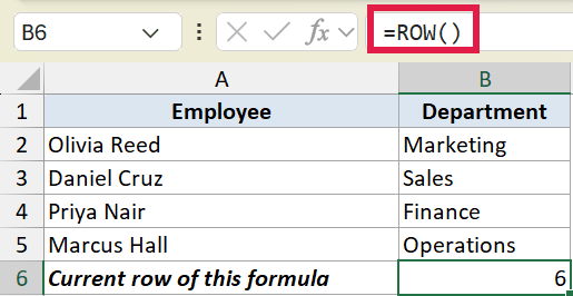
The formula sits in row 6, so it returns 6. With no reference, ROW always reports the row it lives in.
This is handy when a formula needs to know its own position, like subtracting a header offset to turn row numbers into a 1, 2, 3 count.
Example 2: Return the Row Number of a Specific Cell
Here’s another practical scenario.
Below is a small orders table with order IDs in column A and amounts in column B.
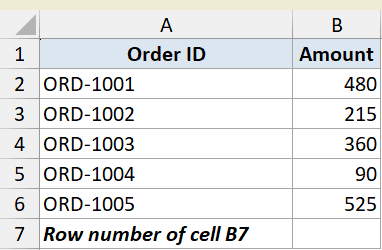
This time we want the row number of a particular cell, B7, rather than the cell the formula sits in.
Here is the formula:
=ROW(B7)
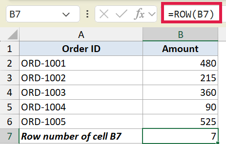
ROW reads the reference and returns 7, because B7 is on row 7. The column letter does not matter. ROW only cares about the row.
Pro Tip: To get a cell’s column position instead of its row, use the COLUMN function. It works exactly the same way, just along the horizontal axis.
Example 3: Generate Serial Numbers That Spill
Let’s put ROW to work on something you will actually use often.
Below is a product list in column B, with an empty Serial No. column in A waiting to be numbered.
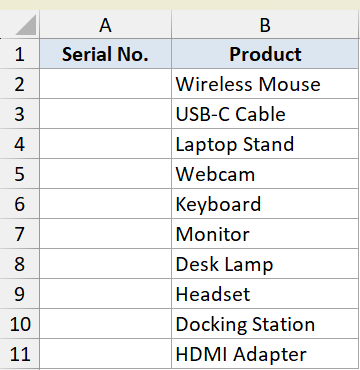
We want a clean 1 to 10 serial number next to each product, in one formula that fills the whole column.
Here is the formula:
=ROW(A2:A11)-1
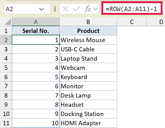
When you give ROW a range, it returns an array of every row number in that range. So ROW(A2:A11) gives 2, 3, 4, all the way to 11.
Subtracting 1 shifts that to 1, 2, 3, up to 10. In Excel 365 the result spills down the column from the single formula in A2.
The numbers stay correct even if you sort the product list, since they are tied to row position, not the data. This is one of the cleanest ways to enter sequential numbers in Excel.
Pro Tip: In Excel 365 you can get the same 1..10 list with the SEQUENCE function, like `=SEQUENCE(10)`, which reads more clearly for plain numbering. ROW is still worth knowing because it keeps working in older Excel versions and inside Tables, where SEQUENCE returns a #SPILL! error.
Example 4: Use ROW as a Dynamic Index in a Lookup
Let’s step it up with a more useful pattern.
Below is a ranked list of cities in column A, with an empty column B where we want to pull them in order.
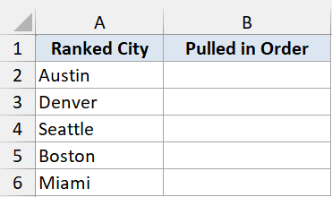
We want column B to fetch the 1st city, then the 2nd, then the 3rd, without typing position numbers by hand.
Here is the formula:
=INDEX($A$2:$A$6,ROW()-1)
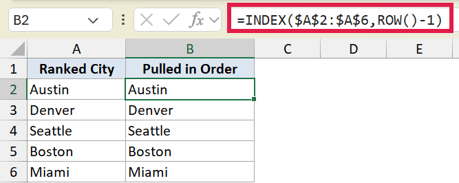
The INDEX function needs a position number, and ROW()-1 supplies it automatically. In B2 the row is 2, so ROW()-1 is 1, and INDEX returns the first city.
As you fill the formula down, ROW()-1 becomes 2, then 3, and so on. Each row pulls the next item with no hard-coded numbers to maintain.
This is the trick behind a lot of “pull every Nth item” and “reshuffle a column” formulas.
Example 5: Flag Every Other Row for Shading
Here’s a classic use that shows up everywhere.
Below is a list of invoice numbers in column A, with an Even Row? column in B we want to fill with a TRUE or FALSE flag.
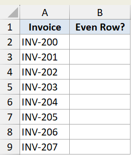
We want each row to report whether it sits on an even-numbered row, which is the test behind banded row shading.
Here is the formula:
=MOD(ROW(),2)=0
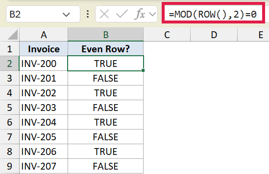
MOD divides the row number by 2 and returns the remainder. Even rows leave a remainder of 0, odd rows leave 1, so the test returns TRUE on even rows and FALSE on odd ones.
Drop the same logic into a conditional formatting rule and you get banded rows. It is also the test behind alternate-row highlighting. The same idea drives every-Nth-row selection when you change the divisor.
Pro Tip: `=ISEVEN(ROW())` does the same job and reads a little cleaner than the MOD version. Use ISODD instead if you want to flag the odd rows. The MOD approach still works everywhere and is easy to adapt for every-3rd or every-5th row.
Tips & Common Mistakes
- ROW with no argument returns the row of the formula cell, not row 1. If you want a count starting at 1, subtract the header offset, like ROW()-1.
- ROW only ever returns the row number. To get the column number instead, use COLUMN. To count rows in a range, use ROWS.
- ROW is not volatile, so it does not slow your sheet down the way TODAY or RAND can. It only recalculates when the rows themselves move.
- When numbering a list, ROW-based serials are tied to position, so they stay sequential even after sorting. Hard-typed numbers do not.
ROW looks like a small function, but it does a lot of the heavy lifting behind auto-numbered lists, dynamic lookups, and banded-row formatting. Once you start reaching for ROW()-1 to build indexes and counts, you will spot uses for it all over your sheets.
Related Excel Functions / Articles: