
The REDUCE function in Excel processes an array with a LAMBDA and returns the final accumulated result.
Each step uses the previous result, which lets you build calculations that carry a total or other state through a list.
Unlike SCAN, REDUCE does not return every intermediate step. Its final result can be a single value or an array, depending on the calculation you define.
In this article, I’ll show you how to accumulate values within a budget cap, compound growth rates, and combine filtered names into a summary.
REDUCE Function Syntax in Excel
REDUCE applies a LAMBDA to each item in an array and carries one accumulator from step to step.
=REDUCE([initial_value],array,lambda(accumulator,value,body))
- initial_value (optional) sets the accumulator’s starting value.
- array (required) is the range or array Excel walks through.
- lambda (required) contains exactly two parameters and the calculation Excel repeats.
- accumulator holds the result carried forward from the previous step.
- value is the current item from the array.
- body returns the new accumulator for the next step.
When to Use REDUCE Function
- Apply a rule where each decision depends on the amount, text, or array already accumulated.
- Compound a series of rates into one ending balance.
- Keep the longest, shortest, or otherwise best value found so far.
- Build one text result from a filtered list.
- Grow an array when each source item needs custom handling.
Example 1: Add Up a Column With REDUCE
A plain total makes the accumulator easy to follow.
Below is the dataset. Columns A and B contain six months and their deposit amounts.
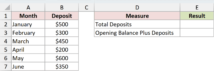
We want to add all six deposits, starting the accumulator at zero.
Here is the formula:
=REDUCE(0,B2:B7,LAMBDA(acc,val,acc+val))
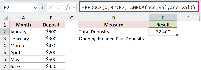
The accumulator starts at 0, then becomes 500, 800, 1,250, 1,450, 2,050, and finally 2,400.
The result in E2 is $2,400.
Now let’s start with an opening balance of $1,200 before adding the deposits.
Here is the second formula:
=REDUCE(1200,B2:B7,LAMBDA(acc,val,acc+val))
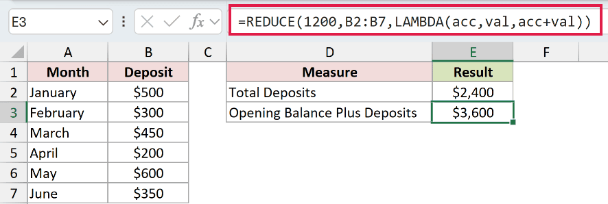
This time, the accumulator begins at 1,200. The same six deposits take it to $3,600 in E3.
Pro Tip: SUM is shorter and faster for a plain total. Use REDUCE when the next step needs the previous result, and use SCAN when you need every running result.
Example 2: Stop at a Budget Cap
Here’s a case where the previous result changes the next decision.
Below is the dataset. Columns A through C list seven requests. The $5,000 Budget Cap in F2 is an input you type.
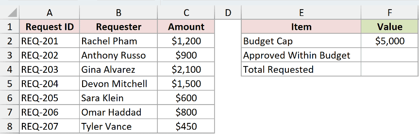
We want to approve each request only when it still fits within the cap.
Here is the REDUCE formula:
=REDUCE(0,C2:C8,LAMBDA(acc,val,IF(acc+val<=$F$2,acc+val,acc)))
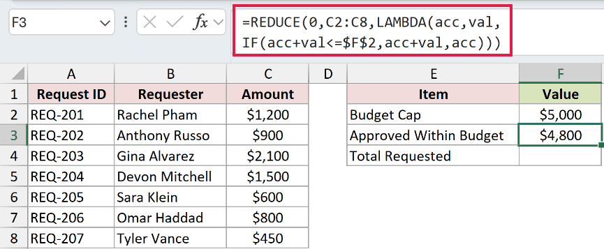
The accumulator reaches 4,200 after three approvals. It refuses $1,500, accepts $600, then refuses $800 and $450 because each would exceed the cap.
The approved total in F3 is $4,800.
For context, we can also add every requested amount without applying the cap.
Here is the SUM formula:
=SUM(C2:C8)
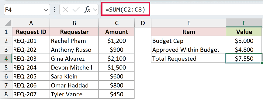
The total requested in F4 is $7,550. The difference shows how much the step-by-step approval rule leaves out.
This is where REDUCE earns its place. A normal conditional total evaluates rows independently, but this rule depends on how much has already been approved.
Example 3: Compound Annual Growth Rates
A portfolio balance shows how the accumulator carries through changing yearly rates.
Below is the dataset. Columns A and B show six years of growth rates. The $25,000 Starting Portfolio in E2 is an input you type.
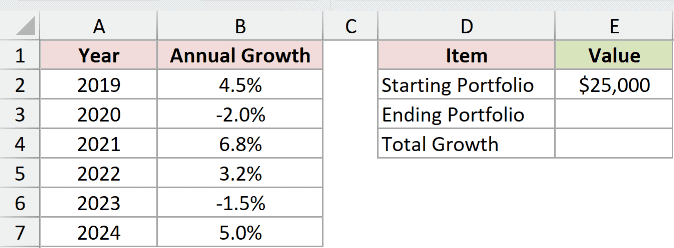
We want each year’s rate to update the balance produced by the previous year.
Here is the REDUCE formula:
=REDUCE(E2,B2:B7,LAMBDA(acc,val,acc*(1+val)))
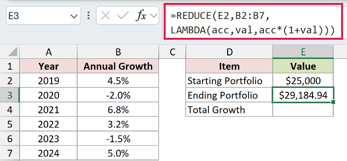
The accumulator starts with the value in E2. Each step multiplies the current balance by one plus that year’s growth rate.
After all six rates, E3 returns an ending portfolio of $29,184.94.
We can then compare that ending value with the typed starting value.
Here is the total growth formula:
=E3/E2-1
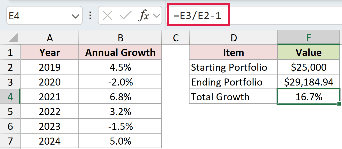
The result in E4 is 16.7% after formatting.
Pro Tip: PRODUCT is shorter when every year follows the same multiplication rule. REDUCE becomes useful when a step must skip, cap, or otherwise react to the balance already accumulated.
Example 4: Find Longest and Shortest Text
The accumulator doesn’t have to be a number. It can keep the best text value found so far.
Below is the dataset. Columns A and B contain eight account IDs and customer names.
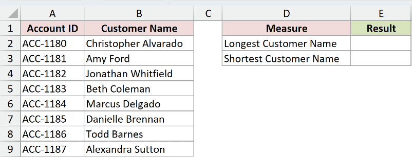
First, we want to return the longest customer name in the list.
Here is the formula:
=REDUCE("",B2:B9,LAMBDA(acc,val,IF(LEN(val)>LEN(acc),val,acc)))
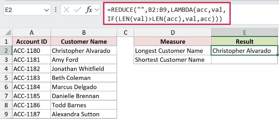
The accumulator starts as empty text. It keeps the current name only when that name is longer than the one already stored.
E2 returns Christopher Alvarado.
Next, we’ll seed the accumulator with B2 and check the remaining names in B3:B9.
Here is the shortest-name formula:
=REDUCE(B2,B3:B9,LAMBDA(acc,val,IF(LEN(val)<LEN(acc),val,acc)))
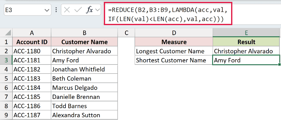
Excel replaces the stored name whenever it finds a shorter one. E3 returns Amy Ford.
With the comma-only form =REDUCE(,B2:B9,LAMBDA(...)), Excel uses the first array item as the starting accumulator and begins the walk with the second item.
An explicit seed is easier to read. Because both tests are strict, the first value wins any length tie.
Example 5: Join and Count Filtered Names
Here’s how REDUCE can work with filtered data and text.
Below is the dataset. Columns A through C list eight territories, sales representatives, and quota statuses.
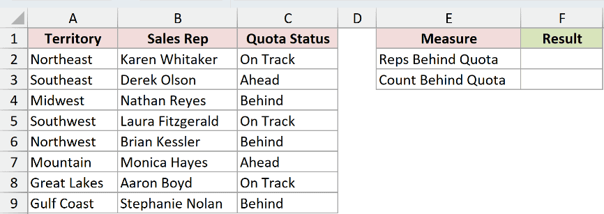
We want one comma-separated list containing only representatives whose status is Behind.
Here is the text formula:
=REDUCE("",FILTER(B2:B9,C2:C9="Behind"),LAMBDA(acc,val,IF(acc="",val,acc&", "&val)))
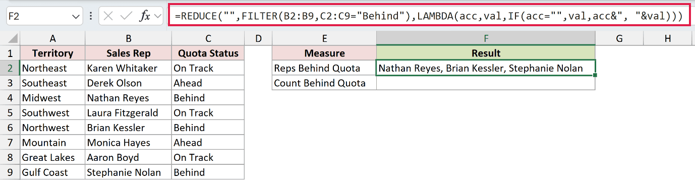
FILTER first supplies the three matching names. The accumulator starts empty, takes the first name, then appends each later name with a comma and space.
REDUCE walks only one array, so FILTER applies the criteria column before the fold rather than inside it.
F2 returns Nathan Reyes, Brian Kessler, Stephanie Nolan.
We can also walk the status column and add one whenever the current value is Behind.
Here is the count formula:
=REDUCE(0,C2:C9,LAMBDA(acc,val,IF(val="Behind",acc+1,acc)))
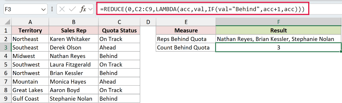
The accumulator remains unchanged for Ahead and On Track. It increases for the three Behind entries, so F3 returns 3.
Pro Tip: TEXTJOIN handles this join more directly, and COUNTIF handles the count more directly. REDUCE is better when the running text or count changes what happens next.
Example 6: Return an Array With REDUCE
The accumulator can also grow into an array instead of remaining one number or text value.
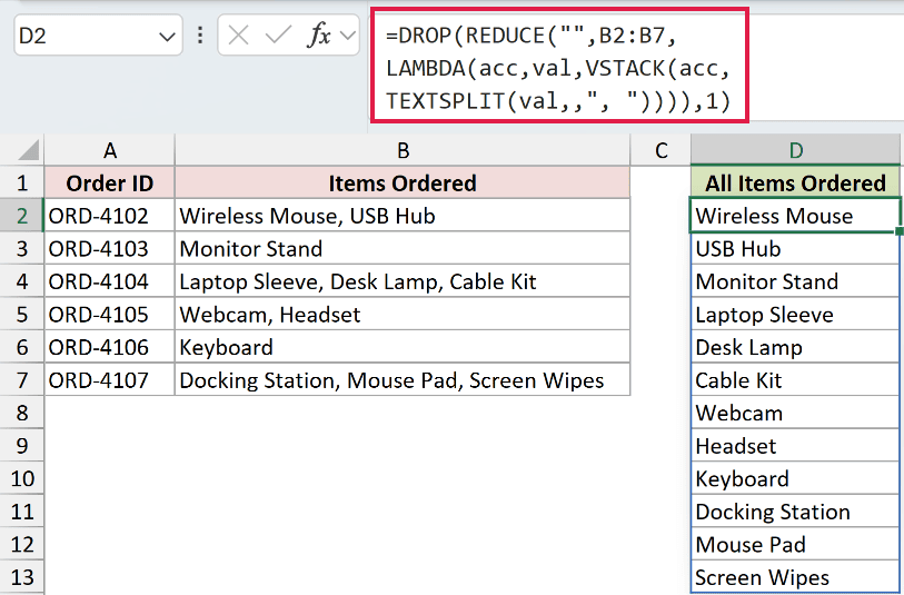
Below is the dataset. Columns A and B contain six order IDs and comma-separated item lists.
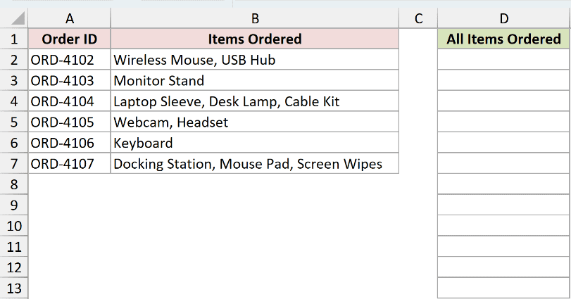
We want to split every order’s items and stack them into one spilled column.
Here is the formula entered once in D2:
=DROP(REDUCE("",B2:B7,LAMBDA(acc,val,VSTACK(acc,TEXTSPLIT(val,,", ")))),1)
The double comma in TEXTSPLIT is intentional. It omits the column delimiter and uses comma plus space as the row delimiter.
Each REDUCE step stacks another split list beneath the growing accumulator. DROP removes the empty seed row, leaving 12 items spilled through D2:D13.
The spill starts with Wireless Mouse and USB Hub. It ends with Docking Station, Mouse Pad, and Screen Wipes.
For this consistent delimiter, TEXTJOIN with TEXTSPLIT is shorter. The REDUCE pattern is useful when each row needs different cleanup, prefixes, or delimiter handling.
Tips & Common Mistakes
- REDUCE works in Microsoft 365, Excel 2024, and Excel for the web. Excel 2021 and earlier return #NAME?.
- A REDUCE LAMBDA needs exactly two parameters in accumulator, value order. Incorrect parameters return #VALUE!.
- Parameter names are your choice, but each name used in the body must match its declaration.
- Start addition at 0 and multiplication at 1. A multiplication fold starting at 0 stays zero at every step.
- REDUCE sees only the current value and accumulator. It cannot directly see a row index or neighboring columns. Filter first, or walk indexes with SEQUENCE and retrieve values with INDEX.
- Built-in functions such as SUM, SUMPRODUCT, TEXTJOIN, COUNTIF, and PRODUCT are usually faster and shorter when no step depends on the previous result.
- REDUCE normally returns one final value. Example 6 spills because its accumulator is deliberately built as an array.
- If you need every intermediate accumulator, use SCAN instead of REDUCE.
- In split-and-stack formulas, split on the comma alone, then trim the pieces with
TRIM(TEXTSPLIT(val,,","))so missing or inconsistent spaces do not prevent a split.
REDUCE is worth reaching for when the next decision depends on what has already been accumulated.
Example 2 is the pattern to revisit when each step must react to the amount accumulated so far.
Related Excel Functions / Articles:
