
Excel formulas don’t have a FOR or WHILE loop like VBA does.
But you can still make a formula repeat a calculation for every character, every row, or every step of a running total.
You do it by handing the formula a list of positions.
Or you use one of the newer LAMBDA helper functions, which walk through an array one item at a time.
In this article, I’ll show you how to loop through the characters in a cell, through each row of a table, across a rows-and-columns grid, and through a running balance.
Method #1: Using SUMPRODUCT With ROW and INDIRECT
This method loops through every character in a cell, and it works in every version of Excel.
ROW and INDIRECT build a list of positions, and the formula checks each one.
Below I have a dataset with order codes in column A. I want to count how many digits each code has.
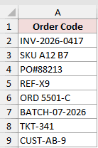
Here is the formula I entered in cell B2 and copied down to B9:
=SUMPRODUCT(--ISNUMBER(--MID(A2,ROW(INDIRECT("1:"&LEN(A2))),1)))
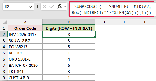
For INV-2026-0417, it returns 8, because the code has eight digits (2026 and 0417).
How does this formula work?
LEN(A2) counts the characters in the code. INV-2026-0417 has 13, so “1:”&LEN(A2) builds the text “1:13”.
INDIRECT turns that text into a real reference to rows 1 through 13. ROW then returns those row numbers, which gives you the list 1 to 13.
MID pulls out one character at each of those 13 positions. So MID runs once for every number in the list, and that’s your loop.
The double minus (–) in front of MID tries to turn each character into a number. Digits convert fine, while letters and dashes return an error.
ISNUMBER returns TRUE for the digits and FALSE for the errors. The outer double minus turns those into 1s and 0s, and SUMPRODUCT adds them up.
I used SUMPRODUCT instead of SUM because it handles arrays in older Excel without pressing Control + Shift + Enter.
Note: INDIRECT is a volatile function, so this formula recalculates every time anything in the workbook changes. On a few hundred rows that’s fine, but on a big sheet it can slow things down.
Method #2: Using the SEQUENCE Function
If you have Excel 2021 or later, there’s a shorter way to build the list of positions. SEQUENCE creates it directly, so you don’t need ROW and INDIRECT.
Below I have the same order codes in column A, with the Method #1 results in column B. I want to count the digits again with SEQUENCE.
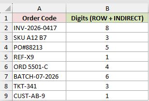
Here is the formula I entered in cell C2 and copied down to C9:
=SUM(--ISNUMBER(--MID(A2,SEQUENCE(LEN(A2)),1)))
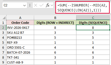
The results match column B. SKU A12 B7 returns 3, PO#88213 returns 5, and REF-X9 returns 1.
How does this formula work?
SEQUENCE(LEN(A2)) returns the numbers 1 to 13 for INV-2026-0417. That’s the same list ROW and INDIRECT built in Method #1, just in one step.
The MID and ISNUMBER part works exactly as before. SUM can add up the array here, because Excel versions with SEQUENCE handle arrays without Control + Shift + Enter.
Since SEQUENCE isn’t volatile, this version also avoids the extra recalculation that INDIRECT causes.
Note: SEQUENCE is available in Excel 2021, Excel 2024 and Microsoft 365. In older versions, this formula returns a #NAME? error, so stick with Method #1.
Method #3: Using the BYROW Function
Here’s another kind of loop. Instead of going through characters, BYROW goes through a table one row at a time and runs the same calculation on each row.
Below I have a dataset with quarterly sales for eight sales reps. I want to find the best quarter for each rep.
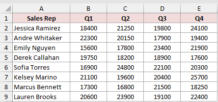
Here is the formula I entered in cell G2:
=BYROW(B2:E9,LAMBDA(r,INDEX(B1:E1,XMATCH(MAX(r),r))))
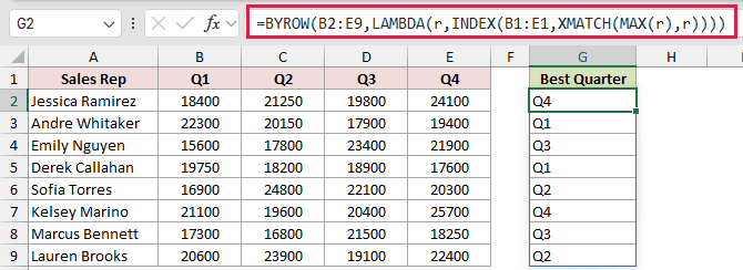
You only enter it once. The results spill down the column automatically, so Jessica Ramirez gets Q4 and Andre Whitaker gets Q1.
How does this formula work?
BYROW takes the range B2:E9 and passes it to the LAMBDA one row at a time.
Inside the LAMBDA, r is the current row, like 18400, 21250, 19800 and 24100 for Jessica.
MAX(r) finds the biggest sale in that row. XMATCH then returns its position within the row, which is 4 for Jessica.
INDEX uses that position to pick the matching header from B1:E1, so position 4 returns Q4.
Note: If a rep has the same top sale in two quarters, XMATCH returns the first match, so the formula shows the earlier quarter.
Method #4: Using the MAKEARRAY Function
Sometimes you need a loop inside a loop, going through every row and every column of a grid. MAKEARRAY does this in a single formula.
Below I have a starting amount of $1,000 in cell B1.
I want to see how it grows over 1, 2, 3, 5 and 10 years at interest rates from 4% to 7%, filling the empty grid in B4:E8.
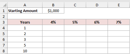
Here is the formula I entered in cell B4:
=MAKEARRAY(5,4,LAMBDA(r,c,$B$1*(1+INDEX(B3:E3,c))^INDEX(A4:A8,r)))
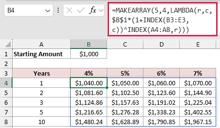
It fills the whole 5 by 4 grid at once. For example, $1,000 at 7% for 10 years grows to $1,967.15.
How does this formula work?
MAKEARRAY(5,4,…) builds a grid with 5 rows and 4 columns. For each cell, it passes the row number (r) and the column number (c) to the LAMBDA.
INDEX(B3:E3,c) picks the interest rate for the current column. INDEX(A4:A8,r) picks the number of years for the current row.
The rest is the regular compound growth calculation. The starting amount is multiplied by (1 + rate) raised to the number of years.
Method #5: Using the SCAN Function
This method is for loops where each step depends on the one before it, like a running balance. SCAN carries the result forward and shows you every step.
Below I have a dataset with monthly deposits in column B and an annual interest rate of 6% in cell F2.
I want the account balance at the end of each month in column C.
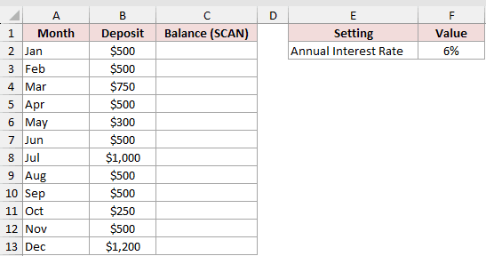
Here is the formula I entered in cell C2:
=SCAN(0,B2:B13,LAMBDA(bal,dep,bal*(1+$F$2/12)+dep))
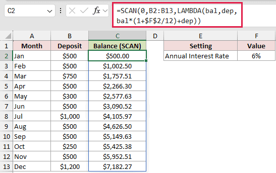
The balance spills down to C13. It starts at $500.00 in January and ends at $7,182.27 in December.
How does this formula work?
SCAN starts with 0 as the opening balance. It then goes through the deposits in B2:B13 one at a time.
In each step, bal is the balance so far and dep is the current deposit.
The LAMBDA adds one month of interest to the balance (the annual rate divided by 12) and then adds the deposit.
In January, that’s 0 plus $500, which gives $500.00. In February, it’s $500 × 1.005 + $500, which gives $1,002.50. SCAN returns the balance after every step.
Method #6: Using the REDUCE Function
REDUCE runs the exact same loop as SCAN. The difference is that it only returns the final result, which is handy when you don’t need the monthly steps.
Below I have the same monthly deposits in column B, the SCAN balances from Method #5 in column C, and the 6% rate in cell F2.
This time I only want the final balance after December, in cell F3.
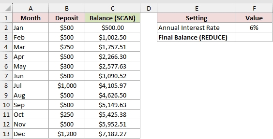
Here is the formula I entered in cell F3:
=REDUCE(0,B2:B13,LAMBDA(bal,dep,bal*(1+$F$2/12)+dep))
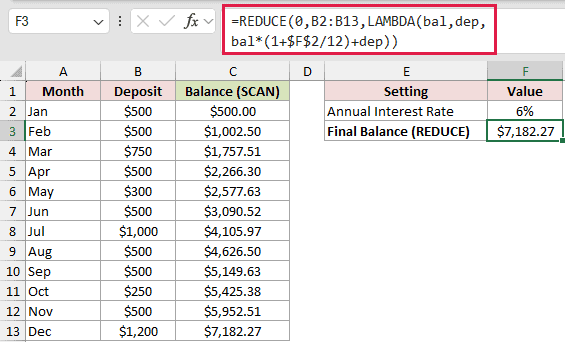
It returns $7,182.27, which is the same as the December balance that SCAN showed in Method #5.
How does this formula work?
The arguments are the same as SCAN’s. REDUCE starts at 0 and walks through B2:B13, adding a month of interest and the deposit at each step.
The only difference is the output. SCAN keeps every intermediate balance, while REDUCE throws them away and keeps only the last one.
Note: BYROW, MAKEARRAY, SCAN and REDUCE are LAMBDA helper functions. They’re available in Excel 2024 and Microsoft 365. In older versions, these formulas return a #NAME? error.
Additional Notes About Looping in Excel Formulas
- A worksheet formula can’t loop forever or stop early like a VBA loop. It always runs through a fixed list, so the size of that list decides how many times it repeats.
- Excel also has a setting called iterative calculation (File > Options > Formulas > Enable iterative calculation). It lets a formula refer to its own cell, but it applies to the whole workbook and is easy to get wrong.
- If a LAMBDA formula returns #VALUE!, check the number of parameters. SCAN and REDUCE need exactly two (the running value and the current item), and MAKEARRAY needs two (row and column).
- Loops over large ranges can get slow. Point the formula at the exact range you need rather than a whole column.
Frequently Asked Questions
Can you write a FOR loop in an Excel formula?
Not directly, because Excel formulas have no FOR or WHILE keyword.
You get the same effect by feeding a formula an array of positions or by using BYROW, SCAN, REDUCE or MAKEARRAY.
How do I loop in a formula without VBA in older Excel?
Use SUMPRODUCT with ROW and INDIRECT, as shown in Method #1. It works in every version and doesn’t need Control + Shift + Enter.
What is the difference between SCAN and REDUCE?
Both run the same step-by-step calculation. SCAN returns the result of every step as a spilled array, while REDUCE returns only the final value.
Can a formula loop until a condition is met?
Not in the way a VBA Do While loop can.
The closest option is a recursive LAMBDA saved in the Name Manager, but for most tasks a fixed loop with SCAN or REDUCE is simpler.
Conclusion
Excel formulas don’t have a real loop statement, but they can still repeat a calculation over characters, rows, grids and running totals.
In this article, I showed you how to loop through the characters in a cell with SUMPRODUCT or SEQUENCE, through each row with BYROW, and across a grid with MAKEARRAY.
I also covered running totals with SCAN and REDUCE.
I hope you found this article helpful.
Other Excel articles you may also like:
