TIME Function in Excel

The TIME function in Excel returns a numeric time value from separate hour, minute, and second inputs.

This is useful when an import splits a timestamp into parts or a formula needs a specific clock time. Apply a time format to display the result.

TIME represents a time of day. Hours beyond a full day roll over, so use duration arithmetic when you need to retain total elapsed hours.

In this article, I’ll show you how to build times from separate columns, interpret 24-hour rollover, and add run times to timestamps.

TIME Function Syntax in Excel

TIME returns a decimal fraction of a day. The cell’s number format controls whether that number appears as a clock time or a decimal.

=TIME(hour, minute, second)

• hour (required) is the hour number, from 0 to 32767.
• minute (required) is the minute number, from 0 to 32767.
• second (required) is the second number, from 0 to 32767.

Values above their natural limits roll into the next unit. For example, 90 minutes becomes 1 hour and 30 minutes.

When to Use TIME Function

• Build valid Excel times from separate hour, minute, and second columns.
• Reconstruct times from fixed-width text codes such as HHMMSS badge stamps.
• Add a numeric run time to a full date and time value.
• Create opening, closing, cutoff, or deadline times inside another formula.
• Normalize extra minutes or seconds when the total stays within one day.

Example 1: Build Times From Hour and Minute Columns

Let’s start with a gym schedule whose time parts arrived in separate columns.

Below is the dataset. Column A lists each class, while columns B and C contain its hour and minute numbers.

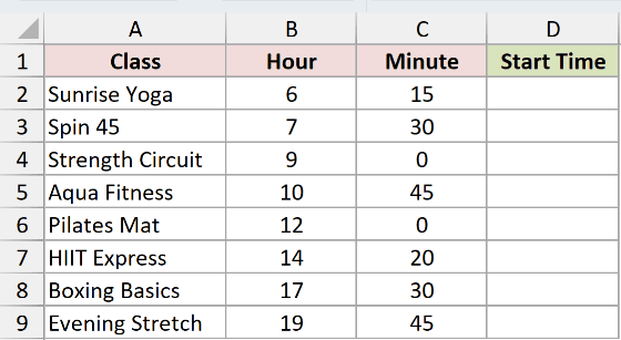
We want one TIME formula to build the start time for every class.

Here is the formula:

=TIME(B2:B9,C2:C9,0)

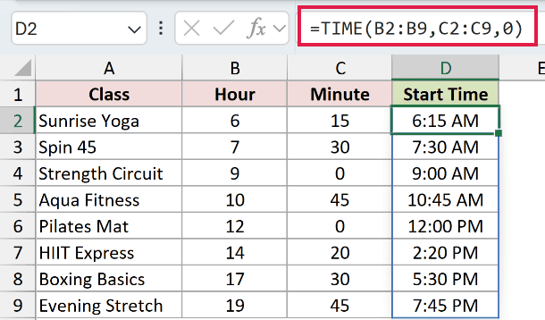
The hour and minute ranges supply the first two arguments. The zero sets every seconds value to zero.

The formula spills from D2 through D9. Sunrise Yoga returns 6:15 AM, Pilates Mat returns 12:00 PM, and Evening Stretch returns 7:45 PM.

TIME stores each result as a decimal fraction of a day. The h:mm AM/PM format controls how that number appears.

Example 2: See TIME Rollover at 24 Hours

This example shows what TIME’s automatic rollover does to minute totals.

Below is the dataset. Column A identifies each machine cycle, and column B contains its recorded minute total.

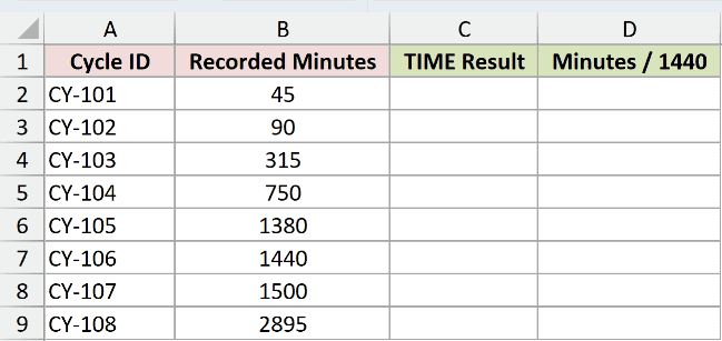
We first want to turn every minute total into a clock time with TIME.

Here is the formula:

=TIME(0,B2:B9,0)

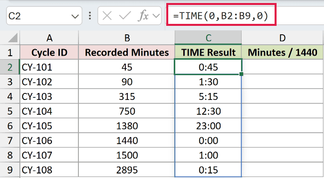
TIME normalizes extra minutes, then wraps the result after 24 hours. That works for clock times but can hide the length of a duration.

To preserve totals of 24 hours or more, use direct division with a duration format for comparison:

=B2:B9/1440

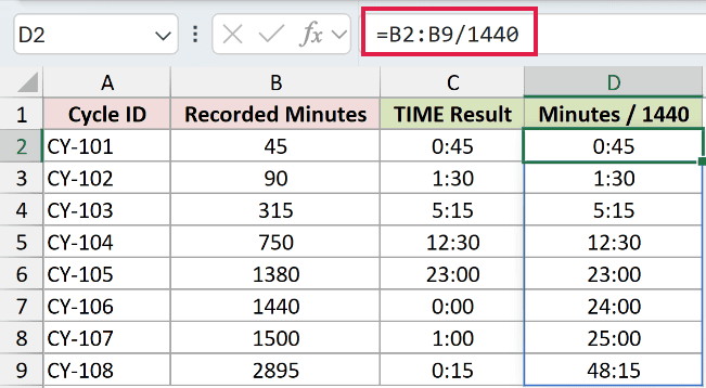
The TIME column uses h:mm, while the comparison column uses [h]:mm. The second formula divides the raw minutes by 1,440 to preserve complete days.

At 1,440 minutes, TIME returns exactly zero because it discards the full day. Changing that cell to [h]:mm would still show 0:00.

The duration formula stores one full day, so its [h]:mm cell shows 24:00.

At 1,500 and 2,895 minutes, the pairs are 1:00 versus 25:00 and 0:15 versus 48:15.

Pro Tip: Use TIME for a time of day. For elapsed time that may exceed 24 hours, use day-fraction arithmetic and format the result as [h]:mm.

Example 3: Convert an HHMMSS Badge Stamp

Now let’s rebuild real times from six-character badge-reader stamps.

Below is the dataset. Column A lists employees, and column B stores their six-character HHMMSS badge stamps as text so leading zeros survive.

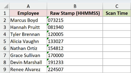
We want to split each stamp into hours, minutes, and seconds, then pass those parts to TIME.

Here is the formula:

=TIME(LEFT(B2:B9,2),MID(B2:B9,3,2),RIGHT(B2:B9,2))

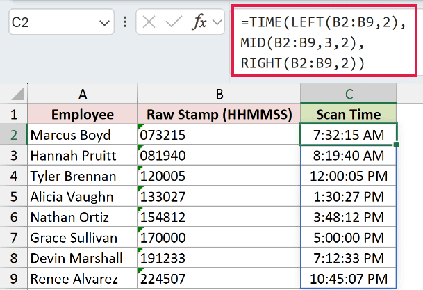
LEFT takes the first two characters, MID takes the middle two, and RIGHT takes the final two. TIME converts those numeric text pieces into times.

The spill starts with 7:32:15 AM for Marcus Boyd, returns 12:00:05 PM for Tyler Brennan, and ends with 10:45:07 PM for Renee Alvarez.

Keep the raw stamps as text. Converting 073215 to a number drops its leading zero, and LEFT(73215,2) returns 73 instead of 07.

TIMEVALUE can parse a time string built with colons, but that route depends on regional settings. TIME takes three numbers, so it avoids that parsing step.

Example 4: Add Run Time to a Timestamp

Next, we’ll add each production run length to its full starting timestamp.

Below is the dataset. It contains batch IDs, starting timestamps, run hours, and run minutes in columns A through D.

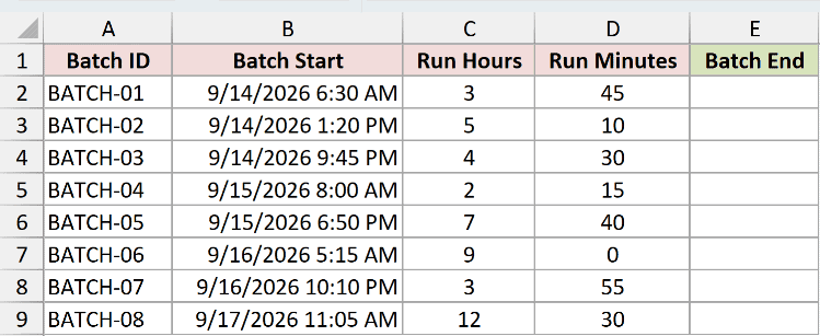
We want one spilling formula to calculate when every batch finishes.

Here is the formula:

=B2:B9+TIME(C2:C9,D2:D9,0)

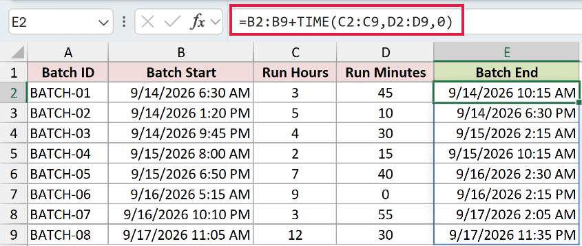
TIME converts each run length into a fraction of one day. Adding that fraction to the full timestamp preserves the date and carries late runs past midnight.

BATCH-03 ends at 9/15/2026 2:15 AM, while BATCH-05 ends at 9/16/2026 2:30 AM.

BATCH-07 ends at 9/17/2026 2:05 AM.

On its own, TIME supplies only a day fraction and sits on Excel’s day zero. The date in column B supplies the calendar portion.

Every run here is under 24 hours because TIME wraps after a full day.

Pro Tip: For a 25-hour run, use =1+TIME(1,0,0) or divide 25 by 24. =TIME(25,0,0) wraps and displays 1:00 AM.

Example 5: Set Opening and Closing Times

Finally, let’s use TIME to create fixed boundaries inside other formulas.

Below is the dataset. Column A contains each chat ID, and column B records when the chat was logged.

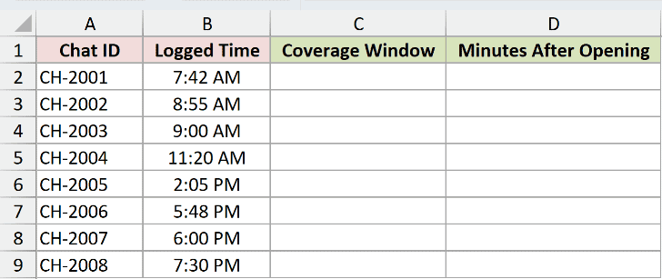
We want to classify each chat against a 9:00 AM opening and a 6:00 PM closing.

Here is the formula:

=IF(B2:B9<TIME(9,0,0),"Before opening",IF(B2:B9>=TIME(18,0,0),"After hours","Open"))

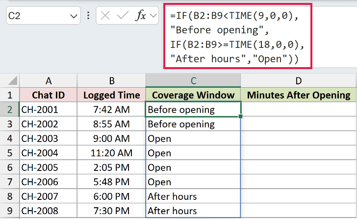
The first test catches times before 9:00 AM. The second catches times at or after 6:00 PM, and everything else returns Open.

The 9:00 AM chat returns Open, while the 6:00 PM chat returns After hours. The opening boundary is included, but the closing boundary is excluded.

IFS could flatten the nested tests, but TIME would still supply the two boundary values.

To show that TIME returns an ordinary number, we can calculate each chat’s minutes after opening:

=(B2:B9-TIME(9,0,0))*1440

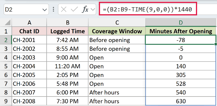
Subtracting the opening time returns a day fraction. Multiplying by 1,440 converts that fraction to minutes.

The 7:42 AM and 8:55 AM chats return -78 and -5 because they arrived before opening. The 9:00 AM chat returns 0.

The later chats return 140, 305, 528, 540, and 630 minutes after opening.

Tips & Common Mistakes

• TIME requires all three arguments. Any negative argument or an argument above 32767 returns #NUM!.
• TIME truncates decimal arguments toward zero. =TIME(8.9,30,0) returns the same 8:30 AM as =TIME(8,30,0).
• A General cell normally changes to h:mm AM/PM when you enter TIME. An existing number format can make the same value appear as a decimal.
• In Excel 2021, Excel 2024, and Microsoft 365, range-based TIME formulas spill. Clear blocked output cells when Excel returns #SPILL!.
• An at sign before TIME forces implicit intersection and reduces a range-based formula to one result. Remove it when you want the full spill.
• In Excel 2019 and earlier, enter the first-row TIME formula and copy it down because those versions do not support dynamic arrays.
• To shift a timestamp backward five hours, subtract TIME(5,0,0) from the timestamp. This keeps the TIME arguments nonnegative.
• COUNTIFS criteria are text, so join the operator to the time value, as in =COUNTIFS(B2:B9,">="&TIME(18,0,0)).

TIME builds a clock time from separate numeric parts. It also works inside formulas that add run times or test time boundaries.

Use TIME for times of day. When a total may exceed 24 hours, preserve the duration with day-fraction arithmetic and an [h]:mm format.

List of All Excel Functions

Related Excel Functions / Articles:

• DATE Function in Excel
• How to Add Hours to Time in Excel?
• How to Add Minutes to Time in Excel?