
The CUMIPMT function in Excel returns the total interest paid over a selected range of loan-payment periods.
It assumes a constant interest rate and regular, equal payments. You can calculate interest for the whole loan or just a portion of its repayment schedule.
Keep the rate and period units consistent. For monthly payments, use a monthly rate and count the periods in months.
In this article, I’ll show you how to calculate loan interest over selected periods, compare loan offers, and separate cumulative interest from principal.
CUMIPMT Function Syntax in Excel
CUMIPMT calculates cumulative interest between two payment periods for a loan with a constant rate and equal payments.
=CUMIPMT(rate, nper, pv, start_period, end_period, type)
- rate (required) is the interest rate per payment period. For monthly payments, divide the annual rate by 12.
- nper (required) is the total number of payments over the entire loan term.
- pv (required) is the original loan amount, entered as a positive number.
- start_period (required) is the first payment period to include. Counting starts at 1.
- end_period (required) is the last payment period to include. Both endpoints are included in the calculation.
- type (required) specifies payment timing:
0for the end of each period or1for the beginning.
The result is negative because interest paid is money leaving your account. A minus sign before CUMIPMT displays that interest as a positive cost.
When to Use CUMIPMT Function
- Calculate the total interest paid over a loan’s full term.
- Find interest paid during a particular year or other payment window.
- Compare interest costs across loan scenarios with different rates and terms.
- Pair interest with principal repayments to check total payments.
- Compare beginning-of-period and end-of-period payment schedules.
Example 1: Calculate Total Car Loan Interest
Let’s start with the full interest cost of a car loan.
Below is the dataset in A1:B3: a $24,000 loan, a 6.90% annual interest rate, and a term of 60 months.
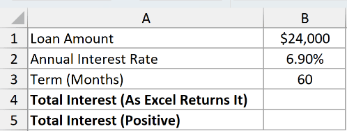
We want to calculate interest across all 60 payments and see why Excel returns a negative number.
Here is the formula for B4:
=CUMIPMT(B2/12,B3,B1,1,B3,0)
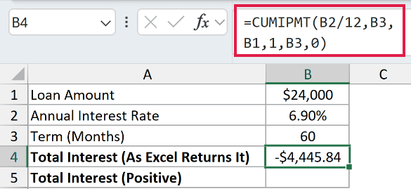
Excel returns -$4,445.84. That minus sign represents a payment out, so it doesn’t mean the loan earns interest for you.
How this formula works:
B2/12converts the annual interest rate to a monthly rate.B3supplies the full term of 60 payments.B1supplies the positive loan amount.1,B3includes every payment from the first through the last.0puts each payment at the end of the month.
To display the same interest as a positive cost, enter this formula in B5:
=-CUMIPMT(B2/12,B3,B1,1,B3,0)
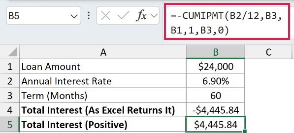
The result is $4,445.84. Only the sign has changed. We’ll use this positive-cost presentation in the remaining examples.
Pro Tip: Keep the loan amount in B1 positive. To change the result’s sign, put the minus before CUMIPMT. A negative pv argument produces #NUM!.
Example 2: Calculate Mortgage Interest by Year
Now let’s break interest into yearly totals without building a monthly repayment schedule.
This example uses a $320,000 mortgage at 6.5% over 30 years. These inputs are entered directly inside the formula.
Below is the dataset in A1:C6. Column A lists years, while columns B and C hold each year’s starting and ending payment months.
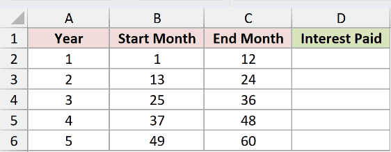
We want the interest paid during each of the mortgage’s first five years.
Here is the formula for D2, which you then copy down to D6:
=-CUMIPMT(6.5%/12,360,320000,B2,C2,0)
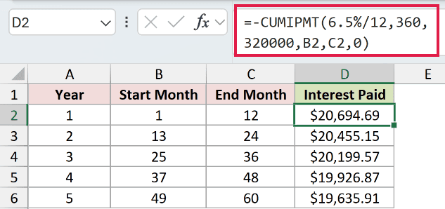
The formula uses 360 monthly payments for the full loan term. The references B2 and C2 select the payment window for each row.
When you copy it down, those references move to the next row. The rate, full term, and loan amount stay constant inside the formula.
The first year returns $20,694.69. The second returns $20,455.15, and the fifth returns $19,635.91.
Interest falls as repayments reduce the outstanding balance. The loan’s early payments carry more interest because the balance is still larger.
Pro Tip: Keep nper at the full loan term, even when you’re calculating one year’s interest. The start and end periods select the year; they don’t shorten the loan.
Example 3: Compare Year One and Year Five
You can also compare two payment windows without calculating the years between them.
Below is the dataset in A1:B3: a $48,000 student loan balance, a 6.80% annual rate, and a 120-month term.
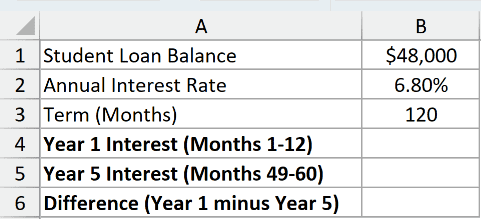
We want to compare interest in the first and fifth repayment years, then calculate the difference.
Here is the formula for the first year’s interest in B4:
=-CUMIPMT(B2/12,B3,B1,1,12,0)
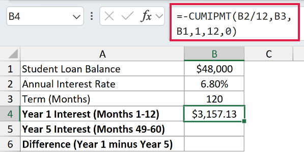
This includes months 1 through 12 and returns $3,157.13.
For the fifth year’s interest, enter this formula in B5:
=-CUMIPMT(B2/12,B3,B1,49,60,0)
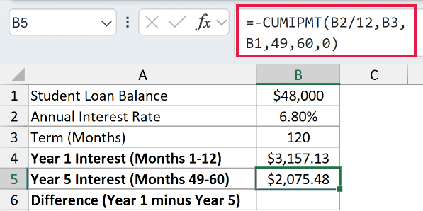
Months 49 through 60 cover the fifth repayment year. The result is $2,075.48, using the same original balance and full loan term.
To calculate how much lower the fifth year’s interest is, enter this formula in B6:
=B4-B5
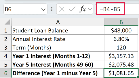
The difference is $1,081.65. Changing the payment window lets you compare specific parts of the same loan.
These are repayment years counted from the first payment. They aren’t automatically calendar years, so choose the periods that match your reporting window.
Example 4: Compare Five Loan Offers
A lower interest rate doesn’t always mean less total interest when the repayment terms differ.
Below is the dataset in A1:D6, with five illustrative lender offers: lender name, annual rate, term in months, and loan amount.
The principal is held constant at $32,000 for every offer, so this comparison isolates the effects of rate and term.
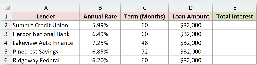
We want to compare total interest over each offer’s full repayment term.
Here is the formula for E2, which you then copy down to E6:
=-CUMIPMT(B2/12,C2,D2,1,C2,0)
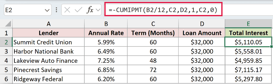
Each row supplies its own rate, term, and loan amount. The term in column C also sets the final payment period.
The 5.99% offer over 60 months returns $5,110.05. But the 7.25% offer over 48 months returns $4,959.85.
Despite its higher rate, the shorter loan accumulates less interest. The 6.85% offer over 72 months has the highest total here, at $7,115.17.
CUMIPMT calculates one row at a time, so copying the formula down is the standard method for this comparison.
Pro Tip: This column compares interest only. Use PMT to compare monthly payments too, and account for any fees separately before comparing the overall cost.
Example 5: Split Interest and Principal
Let’s check how interest and principal fit together across all payments.
Below is the dataset in A1:B3: an $18,000 loan, a 7.25% annual interest rate, and a term of 48 months.
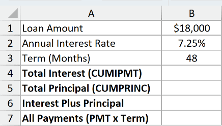
We want to calculate interest and principal separately, then check their sum against the total payments calculated with PMT.
Here is the formula for total interest in B4:
=-CUMIPMT(B2/12,B3,B1,1,B3,0)
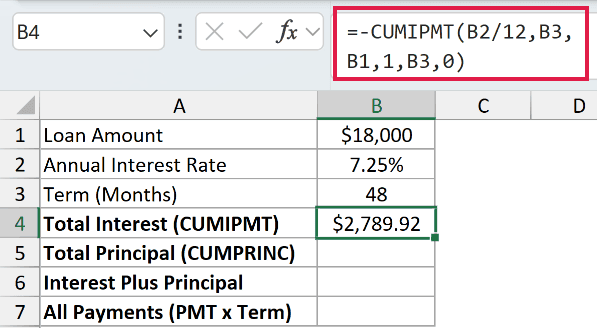
The total interest is $2,789.92.
For the principal repaid, enter this CUMPRINC formula in B5:
=-CUMPRINC(B2/12,B3,B1,1,B3,0)
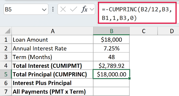
CUMPRINC returns $18,000.00, matching the original loan amount. It’s CUMIPMT’s principal counterpart, and both formulas use the same payment window.
To add the two components, enter this formula in B6:
=B4+B5
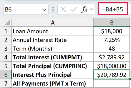
Interest plus principal comes to $20,789.92.
For an independent check using the monthly payment, enter this formula in B7:
=-PMT(B2/12,B3,B1)*B3
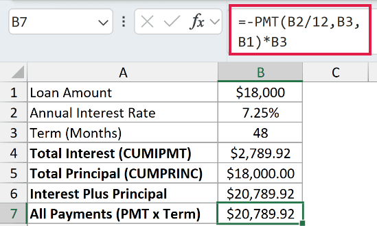
PMT calculates the monthly payment, and multiplying by B3 covers all 48 payments. This also returns $20,789.92, matching the combined total.
Notice that CUMIPMT never asks you to enter the monthly payment. It calculates the interest from the rate, term, loan amount, and payment timing.
Example 6: Change the Payment Timing
Finally, let’s see what the required type argument changes.
Below is the dataset in A1:B3: $15,000 financed at a 5.90% annual interest rate over 36 months.
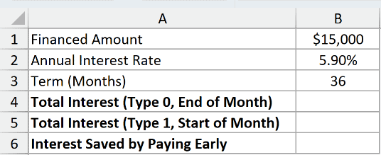
We want to compare total interest when payments fall at the end of each month versus the beginning.
Here is the end-of-month formula for B4, using type 0:
=-CUMIPMT(B2/12,B3,B1,1,B3,0)
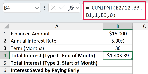
With end-of-month payments, the total interest is $1,403.39.
For beginning-of-month payments, enter this formula in B5, using type 1:
=-CUMIPMT(B2/12,B3,B1,1,B3,1)
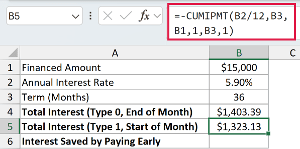
The total interest falls to $1,323.13. Beginning-of-period payments reduce the balance earlier in this payment schedule.
To compare the interest totals, enter this formula in B6:
=B4-B5
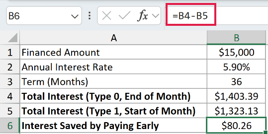
The difference is $80.26 across the full term.
Pro Tip: Choose type to match the payment schedule. Switching it to 1 models beginning-of-period payments throughout the loan; it doesn’t model sending one payment a few days early.
Tips & Common Mistakes
- Keep the rate and term in matching units. Monthly payments need a monthly rate and a term measured in months.
- Supply all six arguments. Unlike PMT, CUMIPMT requires
type; enter0or1deliberately. - Keep
rate,nper, andpvpositive. A zero or negative value for any of these produces#NUM!, including a zero interest rate. - Start counting payments at 1. A starting or ending period below 1, or a start greater than the end, produces
#NUM!. Atypeother than0or1also produces#NUM!. - Keep the original loan amount and full term when selecting a later payment window. The start and end arguments identify which payments to include.
- A negative interest result is Excel’s cash-flow convention. Use a leading minus for a positive cost; ABS is another way to display the magnitude.
- CUMIPMT rejects range arguments. To get a spilled column, use MAP with LAMBDA to call CUMIPMT separately for each input. This requires Microsoft 365 or Excel 2024 and returns
#NAME?in Excel 2021. Otherwise, copy the per-row formula down. - No newer function replaces CUMIPMT. Summing individual IPMT results, with SEQUENCE supplying the payment numbers, can calculate the same end-of-period interest total, but CUMIPMT is more direct. SEQUENCE works in Excel 2021 and later; Excel 2019 and earlier return
#NAME?. - CUMIPMT is available in Excel 2007 and later. The copied-down examples don’t require Microsoft 365.
For your own loan, start by matching the payment frequency and timing. Then choose the first and last payments you want included.
Other Excel articles you may also like:
