
The CUMPRINC function in Excel returns the cumulative principal paid on a loan between two payment periods.
Excel returns that principal as a negative cash flow. When you want a positive amount for reporting, place a minus sign before the function rather than making the loan negative.
In this article, I’ll show you how to handle the negative result, translate calendar dates into payment periods, and check principal against scheduled payments.
CUMPRINC Function Syntax in Excel
The CUMPRINC function uses six required arguments:
=CUMPRINC(rate, nper, pv, start_period, end_period, type)
- rate is the interest rate for each payment period.
- nper is the total number of payment periods for the loan.
- pv is the present value, or original loan amount. Enter it as a positive number.
- start_period is the first payment period included in the calculation.
- end_period is the last payment period included in the calculation.
- type is 0 for payments at the end of each period or 1 for payments at the beginning.
When to Use CUMPRINC Function
- Find how much loan principal was repaid during a particular year or other payment window.
- Build a yearly principal schedule without adding individual PPMT calculations.
- Calculate a remaining loan balance after completed payments.
- Compare principal repayment for end-of-period and beginning-of-period payments.
- Reconcile principal and interest against the total payments for part of a loan term.
Example 1: Handle the Negative Result Correctly
Start with the function’s negative result and the #NUM! error caused by entering the loan amount as negative.
Below are the $345,000 loan amount, 6.75% annual rate, and 30-year term, followed by cells for the raw result, positive amount, and wrong-way test.
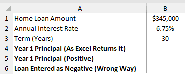
We want to calculate the principal paid during the first year and then display it as a positive amount.
Here is the formula as Excel returns it:
=CUMPRINC(B2/12,B3*12,B1,1,12,0)
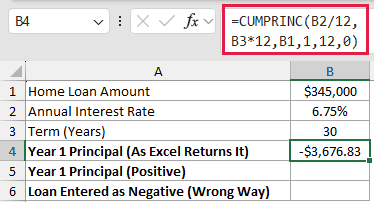
The formula returns -$3,676.83 because Excel treats principal paid as cash leaving the borrower.
Here is the formula for a positive reporting amount:
=-CUMPRINC(B2/12,B3*12,B1,1,12,0)
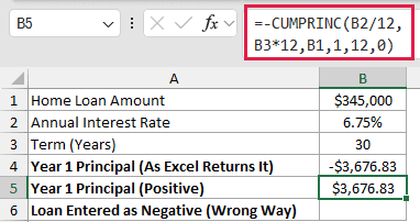
The leading minus sign makes the formula return $3,676.83 as a positive amount without changing the loan input.
Here is the wrong approach, which enters the loan amount as negative:
=CUMPRINC(B2/12,B3*12,-B1,1,12,0)
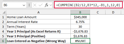
The white B6 cell is deliberately showing the mistake. A negative present value makes CUMPRINC return #NUM! rather than a usable principal amount.
Example 2: Calculate Principal Paid Each Year
A yearly principal schedule puts the payment-window logic to work.
Below is a year column beside the $260,000 loan, 5.99% annual rate, and 15-year term. The empty Principal Paid column will hold the annual amounts.
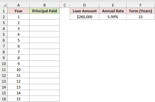
We want each row to calculate the principal repaid during its corresponding loan year.
Enter this formula in B2 and copy it down the column:
=-CUMPRINC($E$2/12,$F$2*12,$D$2,(A2-1)*12+1,A2*12,0)
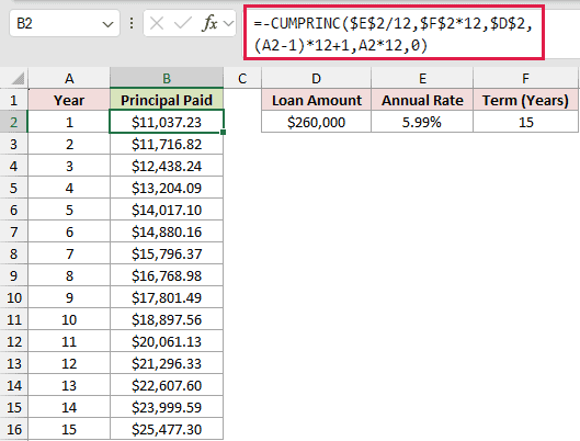
For year 1, (A2-1)*12+1 returns period 1, while A2*12 returns period 12.
For example, the formula returns $11,037.23 in year 1, $16,768.98 in year 8, and $25,477.30 in year 15.
The principal increases as the loan progresses because less of each fixed payment goes toward interest. Together, the 15 yearly amounts total the full $260,000 loan.
A plain period range returns #VALUE! cells, so this schedule copies the formula down one row at a time.
Example 3: Map Calendar Dates to Loan Periods
Here’s how to calculate principal for a calendar year when the loan started partway through the previous year.
The worksheet below pairs a $38,500 auto loan, 6.89% annual rate, and 72-month term with the start and end payment periods. The result cell is empty.
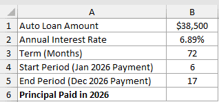
We want the principal paid from January through December 2026.
Here is the formula:
=-CUMPRINC(B2/12,B3,B1,B4,B5,0)
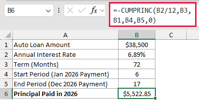
The first payment was in August 2025. That makes January 2026 payment 6 and December 2026 payment 17.
Using those payment numbers, the formula returns $5,522.85 of principal paid during 2026.
This mapping matters because start_period and end_period use payment numbers, not worksheet dates.
Example 4: Find the Remaining Loan Balance
For several borrowers, principal paid also helps reveal the balance still outstanding.
Below is a borrower table listing loan amounts, annual rates, terms, and payments made. The last two columns wait for principal paid and remaining balance.
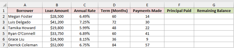
We want to find how much principal each borrower has repaid and how much remains outstanding.
Enter this formula in F2 and copy it down:
=-CUMPRINC(C2/12,D2,B2,1,E2,0)
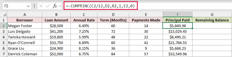
The formula uses Payments Made as the end period, so it includes only payments already completed.
Megan Foster has repaid $5,849.98 in principal, while Derrick Coleman has repaid $32,549.96.
Now subtract the principal paid from the original loan. Enter this formula in G2 and copy it down:
=B2-F2
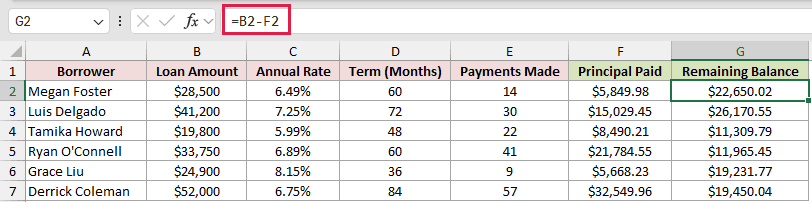
The remaining balances are $22,650.02 for Megan Foster and $19,450.04 for Derrick Coleman.
This calculation assumes the scheduled payments were made as listed. It does not include extra payments, late fees, or other adjustments outside the loan schedule.
Example 5: Compare Payment Timing Types
The required type argument changes when Excel assumes each payment occurs.
The worksheet below uses a $46,000 truck loan, 7.49% annual rate, and 60-month term. Three empty cells will hold the two timing results and their difference.
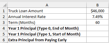
We want to compare the first-year principal when payments occur at the end or beginning of each month.
Here is the formula using type 0 for end-of-month payments:
=-CUMPRINC(B2/12,B3,B1,1,12,0)
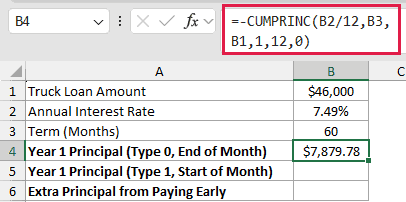
This formula returns $7,879.78 of principal for the first year.
Here is the formula using type 1 for start-of-month payments:
=-CUMPRINC(B2/12,B3,B1,1,12,1)
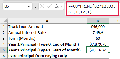
Moving each payment to the beginning of the month increases first-year principal to $8,116.24.
Here is the formula that measures the difference:
=B5-B4
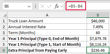
The earlier payment timing moves an extra $236.46 toward principal during the first year.
The type argument accepts 0 or 1. Entering 2 returns #NUM!.
Example 6: Reconcile Principal and Interest
A final check compares principal and interest with the scheduled payments for part of a mortgage.
Below are the $410,000 mortgage amount, 6.25% annual rate, and 360-month term. Four labeled cells wait for principal, interest, their sum, and scheduled payments.
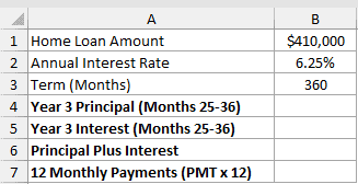
We want to reconcile principal and interest for months 25 through 36.
First, calculate the principal with CUMPRINC:
=-CUMPRINC(B2/12,B3,B1,25,36,0)
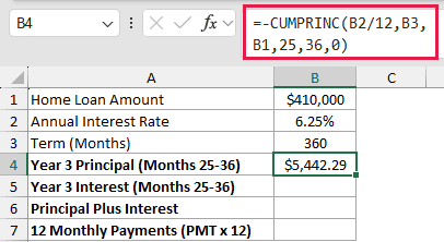
The formula returns $5,442.29 of principal for this payment window.
Next, calculate the interest with CUMIPMT:
=-CUMIPMT(B2/12,B3,B1,25,36,0)
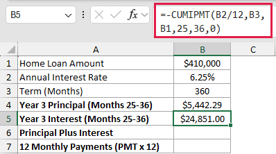
The formula returns $24,851.00 of interest for the same months.
Add the two amounts:
=B4+B5
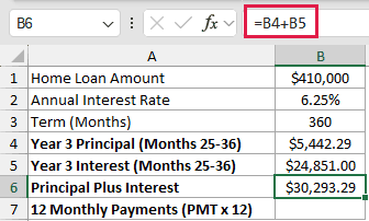
Principal plus interest equals $30,293.29.
Now calculate the same window’s scheduled payments with PMT:
=-PMT(B2/12,B3,B1)*12
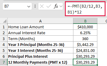
The PMT calculation also returns $30,293.29. That is an exact match with the principal-plus-interest total for the scheduled payments.
This example checks only months 25 through 36. Over the whole term, principal paid equals the $260,000 loan amount shown in Example 2.
Tips & Common Mistakes
- Keep the units consistent. For monthly payments, divide the annual rate by 12 and express the loan term as a total number of months.
- Enter the loan amount as a positive value. Negating the function produces a positive reporting amount, while negating pv returns #NUM!.
- Use whole payment periods, and keep start_period at or before end_period.
- A plain range in a period argument produces #VALUE! cells. In Excel 2021, Excel 2024, or Microsoft 365, adding zero to both period ranges allows the formula to spill.
The payment window does the real work. Translate dates or loan years into the exact start_period and end_period values before calculating.
Related Excel Functions / Articles:
