
The ISPMT function in Excel calculates interest for a specific period of a loan that repays an equal amount of principal each period.
Principal is the borrowed amount you’re paying back. When that repayment stays constant, the outstanding balance falls evenly, so interest and the total payment decrease along the way.
I’ll show you how to number ISPMT periods correctly, build a repayment schedule, and catch payment numbers that fall outside the loan term.
ISPMT Function Syntax in Excel
ISPMT takes the periodic rate, period index, total periods, and original loan amount:
=ISPMT(rate, per, nper, pv)
- rate (required): The interest rate per payment period. For monthly payments, divide the annual rate by 12.
- per (required): The period to calculate, counted from zero. The first payment uses 0, so subtract 1 from an ordinary payment number.
- nper (required): The total number of payment periods, expressed in the same units as the rate.
- pv (required): The present value, or original loan amount. A positive loan amount produces a negative interest result.
For a normal schedule, the period index starts at zero and stops before nper. ISPMT doesn’t enforce that boundary, so an invalid period can still return a number.
When to Use ISPMT Function
- Find the interest portion of a particular payment on an equal-principal loan.
- Build a schedule showing declining interest and total payments while principal repayments stay constant.
- Compare interest under equal-principal and equal-payment repayment methods.
- Calculate interest for loans with different payment frequencies using the same unit-conversion rule.
Example 1: Find Interest for a Specific Month
Let’s start with the period-numbering mistake that’s easy to miss.
Below is the dataset. The card holds the loan amount, annual rate, term, and selected month, with labelled cells for interest and the off-by-one mistake.
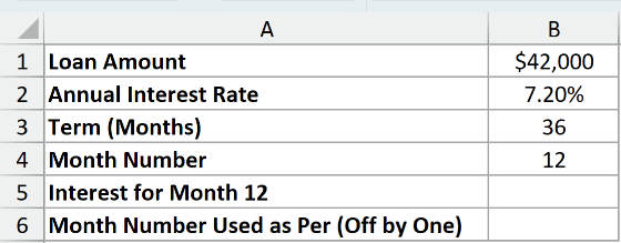
We want the interest for month 12 of a $42,000 loan at 7.20%, repaid over 36 months.
Enter this formula in B5:
=ISPMT(B2/12,B4-1,B3,B1)
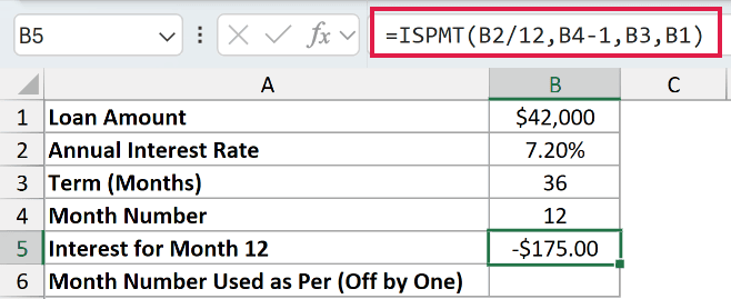
The formula returns -$175.00. The negative sign represents interest paid out when the original loan amount is positive.
B2/12 converts the annual rate to a monthly rate. B4-1 converts the selected month into the zero-based period that ISPMT expects.
Now look at the deliberate mistake in B6, which passes the month number directly:
=ISPMT(B2/12,B4,B3,B1)
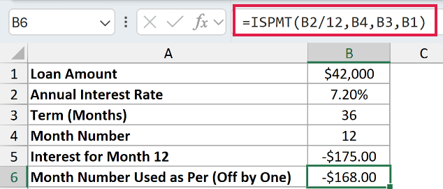
The mistaken formula returns -$168.00. It calculates the following month’s interest, so Excel displays a plausible amount without warning you.
Although the mistake cell has result styling, it isn’t an alternative answer. Keep the subtraction in the per argument when your month labels start at 1.
Example 2: Build an Equal-Principal Payment Schedule
Now let’s calculate interest and total payments for the whole schedule.
Below is the dataset. Column A lists months, B and C have result headers, and E:F contains loan settings, including the monthly principal helper.
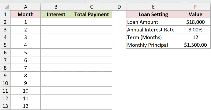
We want the monthly interest and total payment for an $18,000 loan at 8.00% over 12 months.
The settings card already calculates monthly principal in F5 with =F2/F4. That helper returns $1,500.00, the same principal repayment each month.
Enter the interest formula in B2:
=-ISPMT(F3/12,A2:A13-1,F4,F2)
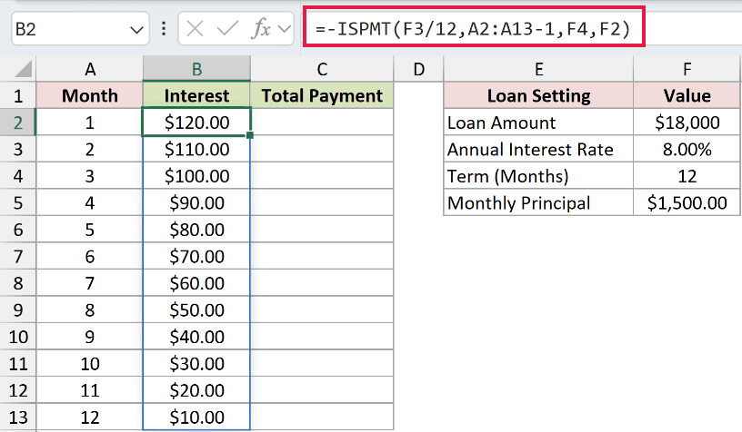
The formula spills into B2:B13, returning an interest amount for each month. The minus sign before ISPMT changes the outgoing interest into positive amounts for the schedule.
Interest starts at $120.00, then $110.00, and finishes at $10.00. It falls evenly because the same principal amount is repaid each month.
Range formulas spill in Excel 2021, Excel 2024, and Microsoft 365. In Excel 2019 and earlier, use a per-row version and fill it down.
Next, enter this formula in C2 to add the fixed principal repayment to each month’s interest:
=F5+B2:B13
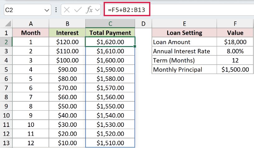
This formula spills into C2:C13. Total payments decline from $1,620.00 to $1,510.00, while the principal portion stays at $1,500.00.
Example 3: Compare ISPMT and IPMT
IPMT calculates a payment’s interest portion when total payments stay fixed. ISPMT assumes equal principal repayments instead.
Let’s compare their interest amounts using identical loan settings.
Below is the dataset. Column A lists months, E:F holds the loan settings, and B:C has headers for ISPMT interest and the IPMT comparison.
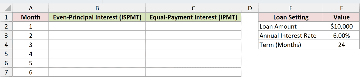
We want to compare the opening months of a $10,000 loan at 6.00% over 24 months.
Enter the equal-principal interest formula in B2:
=-ISPMT(F3/12,A2:A7-1,F4,F2)
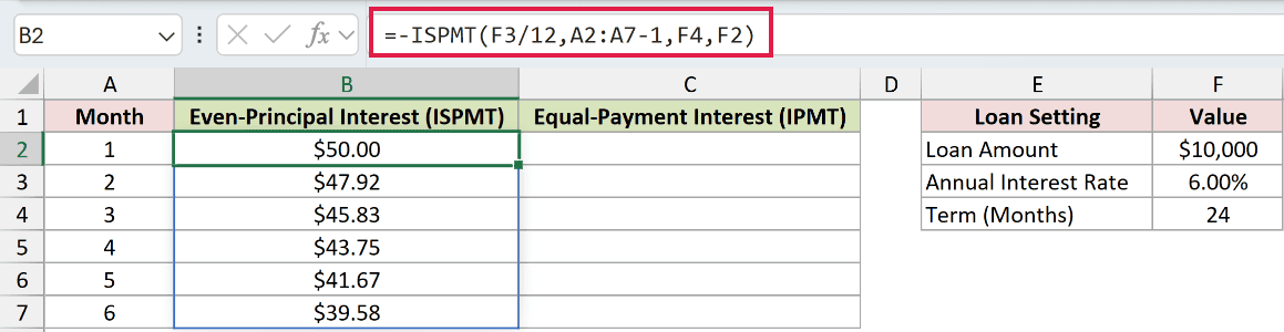
The results spill into B2:B7. Interest starts at $50.00, falls to $47.92 in the next month, and reaches $39.58 in month 6.
For the equal-payment comparison, enter this IPMT formula in C2:
=-IPMT(F3/12,A2:A7,F4,F2)
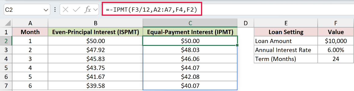
The IPMT comparison spills into C2:C7. It also starts at $50.00, but the next month is $48.03, and month 6 is $40.07.
The opening interest matches because both methods start with the same balance and periodic rate. After that, the principal balances follow different repayment paths.
Notice that the IPMT comparison uses the month numbers directly. IPMT starts counting at 1, while ISPMT starts at 0.
Example 4: Calculate Total Interest Over the Loan
You can also total ISPMT’s period results without building a visible schedule.
Below is the dataset. The card holds the loan amount, annual rate, and term, with labelled cells for total interest, the equal-payment comparison, and the difference.
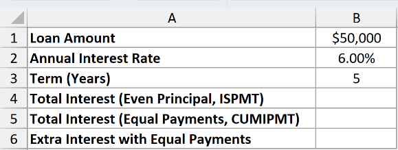
We want total interest on a $50,000 loan at 6.00%, repaid annually over 5 years.
SEQUENCE creates a list of numbers, giving ISPMT every period index to calculate. SUM adds the resulting interest amounts to get the loan’s total interest.
Enter this formula in B4:
=-SUM(ISPMT(B2,SEQUENCE(B3,,0),B3,B1))
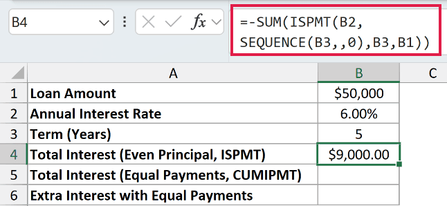
The formula returns $9,000.00 in a single cell.
How this formula works:
SEQUENCE(B3,,0)generates the period indexes starting at zero. The omitted column argument keeps the sequence in a column.- ISPMT calculates interest for those periods using the annual rate and term.
- SUM combines the interest amounts, and the leading minus sign presents the total as positive.
SEQUENCE requires Excel 2021 or later. Although ISPMT calculates an array inside this formula, SUM reduces it to a single total.
CUMIPMT totals interest across specified periods of an equal-payment loan. Here, it lets us compare that total with ISPMT’s equal-principal total.
Enter this formula in B5:
=-CUMIPMT(B2,B3,B1,1,B3,0)
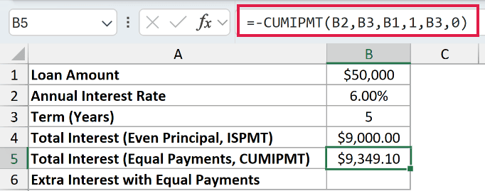
The CUMIPMT comparison returns $9,349.10 for equal payments made at the end of each period.
Calculate the extra interest under the equal-payment comparison in B6:
=B5-B4
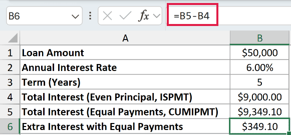
The difference is $349.10. On these loan terms, the equal-payment comparison costs more interest because principal is repaid more slowly at the start.
Example 5: Handle Different Payment Frequencies
The same formula can handle monthly, quarterly, semiannual, and annual payments.
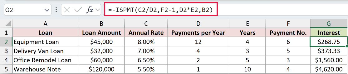
Below is the dataset. Columns B:F list each loan’s amount, annual rate, payments per year, term, and selected payment. Column G has the interest header.

We want the interest for each selected payment using that loan’s own payment frequency.
Enter this formula in G2, then copy it down through G5:
=-ISPMT(C2/D2,F2-1,D2*E2,B2)
How this formula works:
C2/D2converts the annual rate into a rate per payment period.F2-1converts the payment number into ISPMT’s zero-based period.D2*E2converts the term in years into the total number of payments.B2supplies the original loan amount, while the leading minus sign makes the interest positive.
The Equipment Loan returns $268.75, and the Delivery Van Loan returns $373.33. The Office Remodel Loan returns $1,560.00, while the Warehouse Note returns $4,620.00.
Change both the rate and the term when changing payment frequency. Converting only the rate leaves the calculation using inconsistent units.
Example 6: Catch Payment Numbers Outside the Term
ISPMT won’t tell you when a payment number doesn’t belong in the schedule.
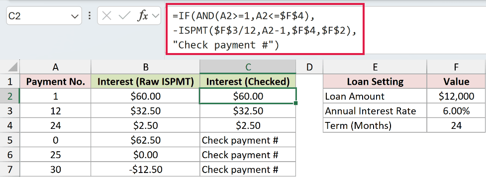
Below is the dataset. Column A contains payment numbers, E:F holds the loan settings, and B:C has headers for the unguarded calculation and checked result.
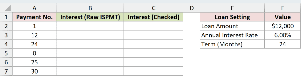
We want to flag invalid payment numbers for a $12,000 loan at 6.00% over 24 months.
First, enter the unguarded formula in B2 and copy it down through B7:
=-ISPMT($F$3/12,A2-1,$F$4,$F$2)
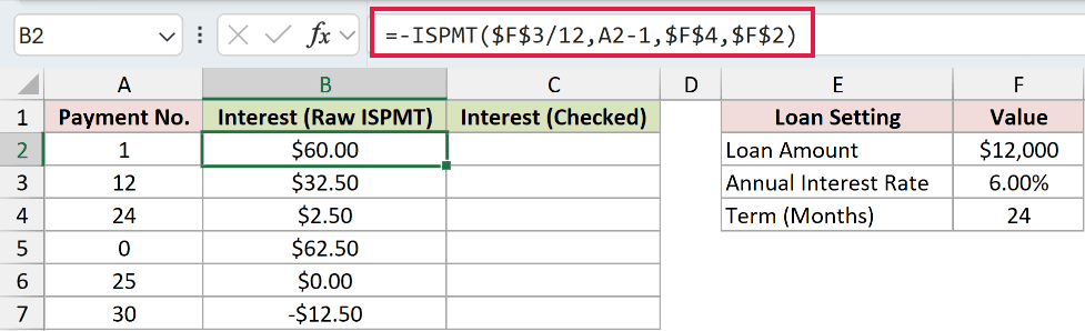
The unguarded column returns $60.00, $32.50, and $2.50 for payments 1, 12, and 24. Those payment numbers belong within the term.
But the unguarded formula also calculates amounts for the invalid rows:
- Payment 0 returns $62.50, even though the payment numbering starts at 1.
- Payment 25 returns $0.00 because its converted period equals the total term.
- Payment 30 returns -$12.50, even though the loan has already ended.
These unguarded results aren’t valid scheduled payments. ISPMT continues the calculation instead of returning an error, so we need to check the payment number ourselves.
To check the payment number first, enter this formula in C2 and copy it down through C7:
=IF(AND(A2>=1,A2<=$F$4),-ISPMT($F$3/12,A2-1,$F$4,$F$2),"Check payment #")
AND checks whether all conditions are met. Here, it checks that the payment number falls between 1 and the term in F4.
IF chooses between two results based on a condition. Here, it runs ISPMT when the payment number passes the check and returns Check payment # otherwise.
The checked column keeps $60.00, $32.50, and $2.50 for valid payments. Each invalid row returns Check payment # instead.
The dollar signs keep the loan settings fixed as you copy down. The payment reference changes with each row so every entry gets its own check.
Tips & Common Mistakes
- Check the repayment structure. ISPMT assumes equal principal repayments, so total payments decrease as interest falls. It doesn’t calculate interest for a loan with fixed total payments.
- Check the starting period. Ordinary payment numbers start at 1, but ISPMT’s
perstarts at 0. Subtracting 1 avoids the silent off-by-one mistake. - Keep the sign intentional. Positive
pvproduces negative interest. Negating the function makes the scheduled expense positive; a negativepvreverses the raw result’s sign. - Validate the term separately. A zero
nperreturns#DIV/0!. The payment-number guard doesn’t replace checking the loan settings. - Use whole payment numbers. ISPMT accepts fractional periods without truncating them. The range guard in Example 6 checks boundaries, so it doesn’t reject decimals within those boundaries.
- Match the rate to the payment period. A zero rate produces zero interest. For other rates, keep the rate and total term in matching units.
Related Excel Functions / Articles:
