
If you want to turn a long row or column into a smaller grid, the WRAPROWS function arranges its values across rows.
In this article, I’ll show you how to control the row width, fill unused cells, and combine WRAPROWS with other functions.
WRAPROWS is a dynamic array function. It spills the reshaped array across the cells below and beside the formula.
WRAPROWS Function Syntax in Excel
The WRAPROWS function uses the following syntax:
=WRAPROWS(vector, wrap_count, [pad_with])
vectoris the one-dimensional row or column you want to reshape.wrap_countis the maximum number of values in each output row.[pad_with]is the optional value used to fill unused cells. If omitted, Excel returns#N/Ain those cells.
When to Use WRAPROWS Function
- Turn a long column into a compact grid for printing or display.
- Break a horizontal list into several rows.
- Replace the default
#N/Apadding with blanks or another marker. - Arrange filtered results into a fixed number of columns.
- Build a numbered grid from a generated sequence.
Example 1: Wrap a Column Into Rows
Let’s start with a basic vertical list.
Below is a column containing ten volunteer names.
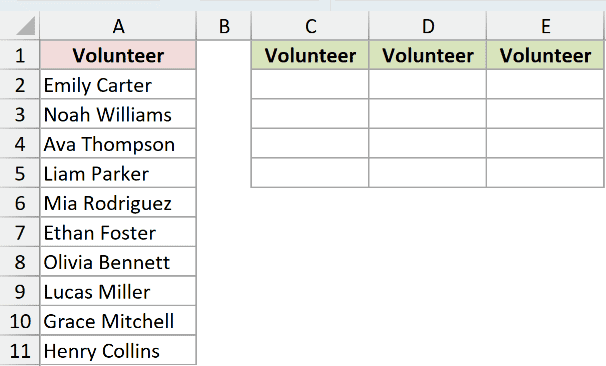
I want to arrange the names in rows containing no more than three volunteers each.
Here is the formula:
=WRAPROWS(A2:A11,3)
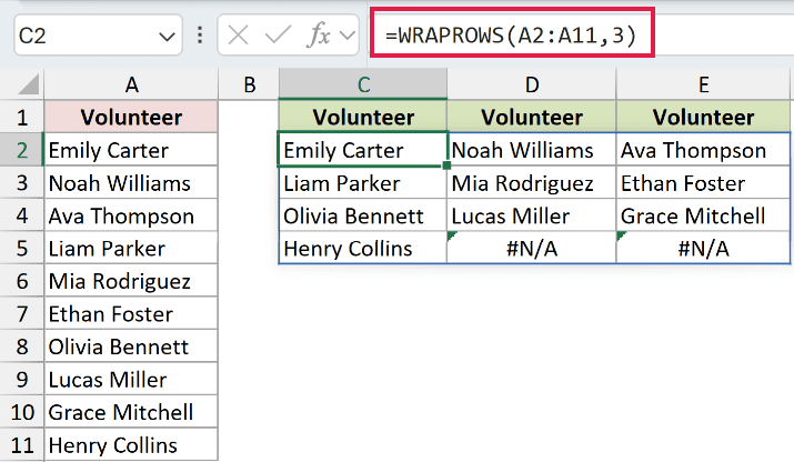
Excel reads down A2:A11 and places each group of three names across one output row.
Ten names need four rows, so the final row contains Henry Collins followed by two #N/A errors.
Those errors are the default padding for cells that have no source value.
Example 2: Replace #N/A With Blanks
You can change the value used to fill the unused cells.
Below is another list of ten team members.
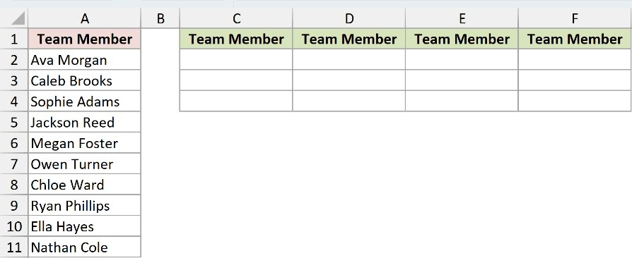
I want to place four names in each row and leave the remaining cells blank.
Here is the formula:
=WRAPROWS(A2:A11,4,"")
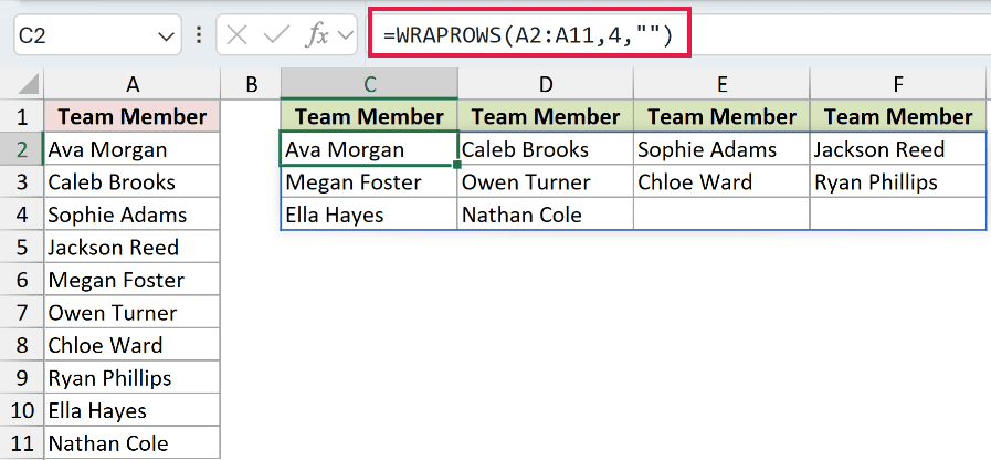
The second argument sets the output width to four values per row.
The empty text string in the third argument replaces the default #N/A padding. The final row therefore shows Ella Hayes and Nathan Cole followed by two blanks.
Pro Tip: The pad_with argument changes only unused cells at the end of the result. It does not replace blanks that already exist in the source vector.
Example 3: Wrap a Horizontal Row
WRAPROWS works with a one-dimensional row as well as a column.
Below is a horizontal list of eight shift codes in B1:I1.

I want to break the codes into rows of three and mark the unused final cell with a hyphen.
Here is the formula:
=WRAPROWS(B1:I1,3,"-")
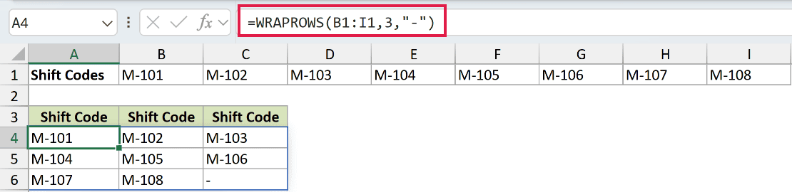
The first row contains M-101 through M-103, and the second contains M-104 through M-106.
The third row contains M-107, M-108, and the hyphen supplied through pad_with.
WRAPROWS accepts only a one-dimensional vector. Passing a source with both multiple rows and multiple columns returns a #VALUE! error.
Example 4: Wrap Filtered Results
You can reshape a filtered list with one formula.
Below is an employee list showing each person’s department. Cell E1 contains Sales, the department I want to return.
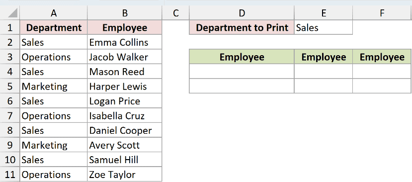
I want to filter the Sales employees and arrange their names across three columns.
Here is the formula:
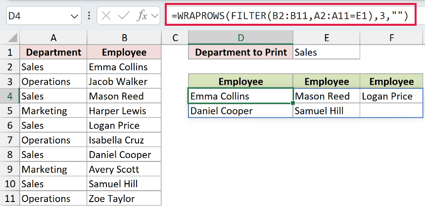
=WRAPROWS(FILTER(B2:B11,A2:A11=E1),3,"")
How this formula works:
- The FILTER function returns the five employees whose department matches Sales in E1.
- WRAPROWS arranges Emma Collins, Mason Reed, Logan Price, Daniel Cooper, and Samuel Hill across rows of three.
- The empty text string fills the sixth output cell with a blank.
Pro Tip: FILTER controls which values enter the result. WRAPROWS only changes how those returned values are arranged.
Example 5: Build a Seven-Column Number Grid
WRAPROWS can also reshape an array created by another dynamic array function.
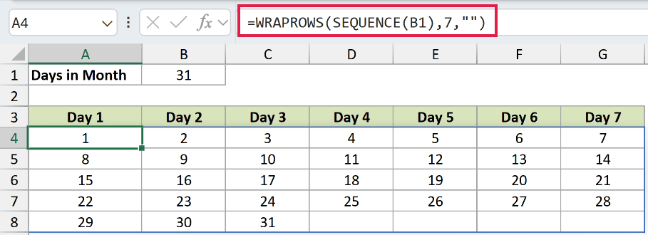
Below is a small setup with the number of days, 31, entered in cell B1.
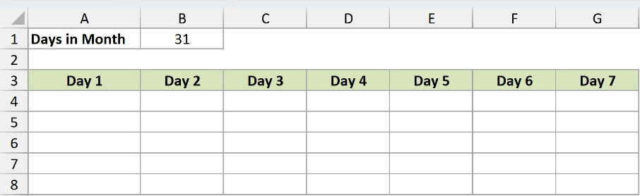
I want to create the numbers 1 through 31 and arrange them in rows of seven.
Here is the formula:
=WRAPROWS(SEQUENCE(B1),7,"")
How this formula works:
- The SEQUENCE function creates a vertical array containing the numbers 1 through 31.
- WRAPROWS places seven numbers in each row, producing five output rows.
- The last row contains 29, 30, and 31, followed by four blank cells.
This creates the numeric part of a month-style grid. It does not assign the numbers to actual dates or weekdays.
Tips & Common Mistakes
- WRAPROWS is available in Microsoft 365 and Excel 2024. Earlier perpetual versions, including Excel 2021, do not support it.
- The source must be a single row or a single column. A two-dimensional source returns a
#VALUE!error. - A
wrap_countbelow 1 returns a#NUM!error. - If you omit
pad_with, Excel puts#N/Ain every unused cell at the end of the returned array. - Keep the output area clear to avoid a
#SPILL!error, and place the formula outside an Excel Table. - Use WRAPCOLS when you want each group to fill down a column before moving to the next column.
I covered how to wrap row and column vectors, control padding, and reshape filtered or generated arrays.
I hope you found this article helpful.
Other Excel articles you may also like:
