
Summing every N rows in Excel lets you pull every third value into one total, or turn monthly sales into separate quarterly totals.
A plain SUM over the whole column adds everything together, so you need a way to pick positions or split the values into groups.
I’ll use SUM with FILTER to add every third row, and BYROW with WRAPROWS for quarterly totals. I’ll also show you alternatives for older Excel versions.
Sum Every Nth Row in Excel
Here I want one total from the third, sixth, ninth, and twelfth values. You skip the values between them rather than adding whole groups.
Method #1: Using SUM and FILTER
I recommend this formula when you want to sum every Nth row in Excel 365, Excel 2021, or later.
Below I have a dataset with 12 months and their sales in A1:B13, from January through December.
I want to add the sales for March, June, September, and December. Those are the third, sixth, ninth, and twelfth values in B2:B13.
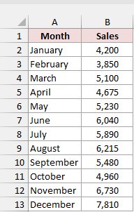
Enter the formula in D2, below the header Every 3rd Row Total.
Here is the formula:
=SUM(FILTER(B2:B13,MOD(SEQUENCE(ROWS(B2:B13)),3)=0))
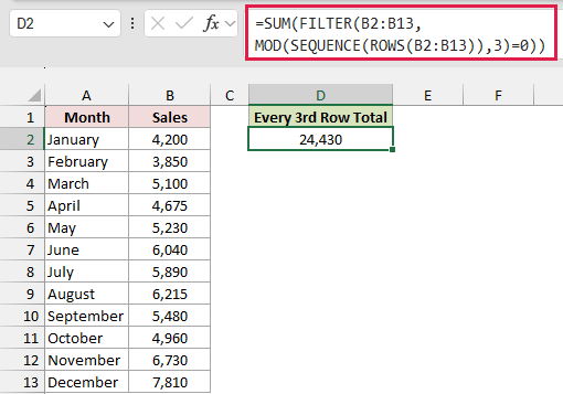
How does this formula work?
You’ll see 24,430 in D2, from adding 5,100 + 6,040 + 5,480 + 7,810.
ROWS(B2:B13) counts the sales rows. There are 12 values, so it returns 12.
SEQUENCE(12) returns the position numbers 1 through 12, one for each value. Positions start at the first sales value, regardless of its worksheet row.
MOD(position,3) returns the remainder after dividing each position by 3. Checking that remainder lets you pick every third position.
You’ll get a remainder of 0 at positions 3, 6, 9, and 12, so MOD(...,3)=0 returns TRUE at those positions.
FILTER keeps the sales where that test returns TRUE. SUM adds those four values and returns one total.
Change the 3 to the interval you need. To sum every other row, use 2 instead; you’ll get 33,550 for this dataset.
Method #2: Using SUMPRODUCT and MOD
If you’re using an older Excel version, you can get the same total with SUMPRODUCT. You can use this formula in every Excel version.
Below I have a dataset with January through December in column A and their sales in B2:B13.
Here I want the total for every third sales value, starting with March and ending with December.
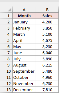
Enter the formula in D2, under Every 3rd Row Total. Press Enter normally; you don’t need Ctrl + Shift + Enter.
Here is the formula:
=SUMPRODUCT((MOD(ROW(B2:B13)-ROW(B2)+1,3)=0)*B2:B13)
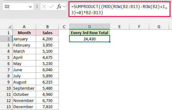
How does this formula work?
You’ll get 24,430, adding the March, June, September, and December sales.
ROW(B2:B13) returns worksheet row numbers 2 through 13. These aren’t the positions within the sales list yet.
Subtracting ROW(B2) and adding 1 turns those numbers into positions 1 through 12. Now your first sales value counts as position 1.
MOD(...,3)=0 identifies positions divisible by 3. It returns TRUE for every third value and FALSE for the others.
When you multiply those tests by B2:B13, TRUE keeps the sales value and FALSE becomes 0. SUMPRODUCT adds the resulting values.
To change the interval, replace the 3 with your N.
Note: Keep -ROW(B2)+1 in the formula so you count from the first sales value. Without it, =SUMPRODUCT((MOD(ROW(B2:B13),3)=0)*B2:B13) returns 22,025. You select worksheet rows 3, 6, 9, and 12, which contain February, May, August, and November.
Sum Every N Rows as Separate Totals in Excel
Here I want a total for each group of three consecutive rows. You add January through March together, then start a new total for April through June.
Method #3: Using BYROW and WRAPROWS
For separate block totals, I recommend this formula in Excel 365 or Excel 2024. You can’t use WRAPROWS in Excel 2021.
You enter one formula, and Excel fills all four totals automatically. That’s called spilling, so you won’t need to copy the formula down.
Below I have a dataset with 12 months and their sales in A1:B13. I want to sum every three rows into quarterly totals.
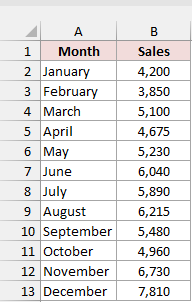
Type Quarter in D1 and Quarterly Sales in E1. Enter Q1 through Q4 in D2:D5, and leave E3:E5 empty for the results.
Enter the formula in E2.
Here is the formula:
=BYROW(WRAPROWS(B2:B13,3,0),LAMBDA(r,SUM(r)))
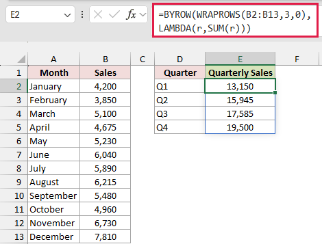
How does this formula work?
You’ll get these quarterly totals in E2:E5:
- Q1: 13,150 for January through March.
- Q2: 15,945 for April through June.
- Q3: 17,585 for July through September.
- Q4: 19,500 for October through December.
WRAPROWS(B2:B13,3,0) arranges the sales into rows of three values. Your 12 values become four rows, each containing one quarter’s sales.
LAMBDA(r,SUM(r)) adds each row. Here, r stands for the row being summed, and LAMBDA defines that calculation.
BYROW runs that calculation on each row of the grid. You get one total per quarter, spilling down the column automatically.
Change the 3 to group your data into blocks of a different size.
If your last block has fewer than N values, you need something to fill the gaps. That’s the third argument in WRAPROWS, called the pad value.
The pad value of 0 won’t change the total. Without a pad value, you’ll get #N/A in the gaps and in the final sum.
For example, change the block size to 5 with these 12 sales values. You’ll get 23,055, then 28,585, then 14,540 for the last two values.
Method #4: Using SUM and OFFSET
For block totals in an older Excel version, you can move the summed range down three rows at a time with OFFSET.
The formula works in every Excel version. Each output row needs its own formula, so you’ll copy it down.
Below I have a dataset with January through December and their sales in A1:B13. I want four quarterly totals, each adding three consecutive sales values.
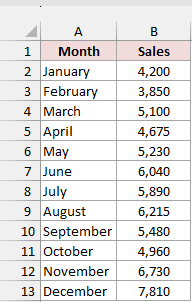
Type Quarter in D1 and Quarterly Sales in E1, then enter Q1 through Q4 in D2:D5.
Enter the formula in E2, then copy it down to E5.
Here is the formula:
=SUM(OFFSET($B$2,(ROWS($E$2:E2)-1)*3,0,3,1))
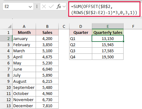
How does this formula work?
After copying down, you’ll see 13,150 for Q1 and 15,945 for Q2. You’ll get 17,585 for Q3 and 19,500 for Q4.
ROWS($E$2:E2) counts the output rows. It returns 1 in E2, 2 in E3, and so on as the range grows.
Subtracting 1 and multiplying by 3 returns 0, 3, 6, and 9. Those numbers tell you how far to move down from B2.
$B$2 keeps the starting cell fixed. OFFSET moves down by the calculated amount and across by 0 columns.
The final arguments, 3 and 1, give you a range three rows tall and one column wide. SUM adds the values in that range.
In E2, you sum B2:B4. In E3, you move down three rows and sum B5:B7, covering April through June.
For a different block size, change both 3s. You need to change the distance between blocks and the height of each summed range.
For a short final block, you’ll still sum a range N rows tall. Keep the cells below your sales list empty so you don’t include unrelated values.
Note: OFFSET recalculates whenever anything in the workbook changes. It’s called a volatile function, and many OFFSET formulas can slow down a large workbook. For a non-volatile alternative, use =SUM(INDEX($B$2:$B$13,(ROWS($E$2:E2)-1)*3+1):INDEX($B$2:$B$13,ROWS($E$2:E2)*3)). INDEX identifies each block’s starting and ending cells. Copy it down for the four complete blocks here.
Additional Notes About Summing Every N Rows in Excel
- These formulas work by position, so sorting the data changes which values occupy every Nth slot or land in each block.
- Hidden and filtered rows still count. These formulas don’t limit the calculation to visible rows.
- Changing
=0to=1in either Nth-row formula starts with the first value. With N = 3, that adds January, April, July, and October, returning 19,725. - Inserting a row inside B2:B13 shifts the later values into different positions, so your block totals can change.
- SUM ignores text in the range. The multiplying SUMPRODUCT formula returns #VALUE! when B2:B13 contains text; use the comma form below to count text as 0.
=SUMPRODUCT(--(MOD(ROW(B2:B13)-ROW(B2)+1,3)=0),B2:B13)
Frequently Asked Questions
You can also adapt these calculations for values across columns or build a summary from numbered groups.
How Do I Sum Every Nth Column Instead of Every Nth Row?
Use COLUMN instead of ROW to count positions across your data. For values in B2:M2, this formula adds every third value:
=SUMPRODUCT((MOD(COLUMN(B2:M2)-COLUMN(B2)+1,3)=0)*B2:M2)
Can I Sum Every N Rows With a Pivot Table?
Yes. First, give each block a group number in a helper column. For the monthly sales example, enter this formula in F2 and copy through F13:
=INT((ROW(B2)-ROW($B$2))/3)+1
You’ll get three 1s, followed by three 2s, and so on. Use those group numbers as the Pivot Table’s row field and sum Sales as values.
If you’d rather calculate a particular group with SUMIF, this formula totals group 2 and returns 15,945:
=SUMIF(F2:F13,2,B2:B13)
Can I Sum Every Nth Row Without FILTER in Excel 365?
Yes. You can arrange values in rows of three, then take the last column. That column contains every third value in this example:
=SUM(TAKE(WRAPROWS(B2:B13,3),,-1))
WRAPROWS makes four rows of three values. TAKE selects the last column using -1, and SUM adds those values, returning 24,430.
How Do I Average Every N Rows in Excel?
For complete blocks, replace SUM with AVERAGE inside Method #3’s LAMBDA. In Method #4, replace the outer SUM with AVERAGE.
For an incomplete final block, don’t keep Method #3’s zero padding. Those added zeros count in the average and lower it.
Use Method #4 for that case, keeping the unused cells below your data empty. AVERAGE ignores those empty cells when calculating the final block.
Conclusion
I’d start with SUM and FILTER for one Nth-row total, or BYROW and WRAPROWS for separate block totals in Excel 365.
For older Excel versions, use SUMPRODUCT for one total and SUM with OFFSET for a total per block.
Other Excel articles you may also like:
