BYCOL Function in Excel

Excel’s BYCOL function applies a LAMBDA calculation to each column of an array and returns one result for every source column.

The results spill horizontally, which makes BYCOL useful for totals, counts, averages, and other column summaries produced by one formula.

BYCOL is available in Microsoft 365 and Excel 2024. It is not available in Excel 2021 or earlier versions.

In this article, I’ll show you how to calculate column totals, count values above a threshold, and average filtered rows with BYCOL.

BYCOL Function Syntax in Excel

The BYCOL function takes an array and a single-parameter LAMBDA.

=BYCOL(array,LAMBDA(column,calculation))

• array is the range or array to process one column at a time.
• column is the single LAMBDA parameter representing the current source column.
• calculation returns one value for that column. BYCOL repeats it for every column in the array.

When to Use BYCOL Function

• Create a horizontal row of totals or averages with one formula.
• Count values that meet a condition in each column.
• Summarize columns after filtering the source rows.
• Use a per-column result vector to return selected headers.
• Stack several column summaries into a small report.

Example 1: Calculate Every Column Total

Let’s start with a horizontal totals row.

Below is a returns table with eight categories across five months and a summary area for the monthly totals.

I want one formula to total each month from January through May.

Here is the formula:

=BYCOL(B2:F9,LAMBDA(c,SUM(c)))

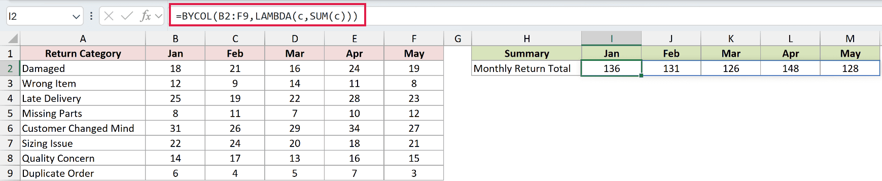
BYCOL passes the January values to c, and SUM(c) returns 136. It repeats the calculation for the remaining month columns.

The five results spill across I2:M2: 136, 131, 126, 148, and 128.

In older Excel versions, you can use =SUM(B2:B9) and copy it across. BYCOL keeps the entire summary row in one formula.

Pro Tip: Keep the cells to the right of the formula empty. Any value inside the intended output range causes a #SPILL! error.

Example 2: Count Values Above a Threshold

Conditional calculations need the full LAMBDA form.

Below is a support backlog table showing eight teams across five weekdays, with a summary row for counts above 20.

I want to count how many teams have more than 20 open tickets on each day.

Here is the formula:

=BYCOL(B2:F9,LAMBDA(c,SUM(--(c>20))))

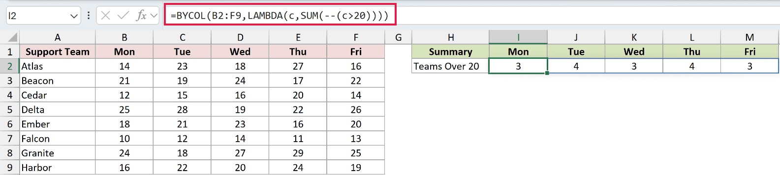
Inside each column, c>20 creates TRUE and FALSE results. The double unary -- converts them to 1 and 0, and SUM counts the 1s.

The formula returns 3, 4, 3, 4, and 3 for Monday through Friday.

Pro Tip: Change >20 to another test, such as >=25 or =0, without changing the rest of the formula.

Example 3: Average Filtered Rows by Column

BYCOL can summarize an array returned by another function.

Below is a regional revenue table, a selected region cell set to West, and four monthly result columns.

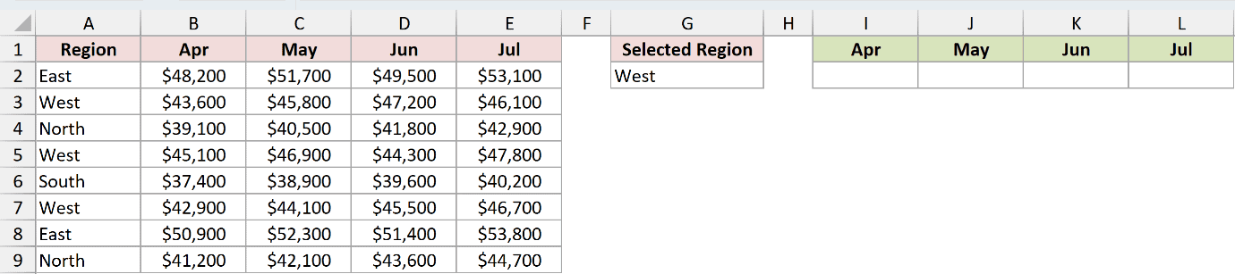
I want the average revenue for each month using only the West rows.

Here is the formula:

=BYCOL(FILTER(B2:E9,A2:A9=G2),LAMBDA(c,AVERAGE(c)))

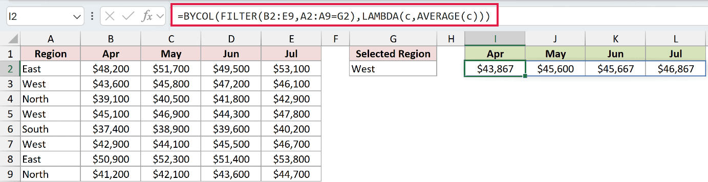
FILTER first returns the three West rows. BYCOL then sends each month column to AVERAGE(c).

The results are $43,867, $45,600, $45,667, and $46,867 after currency formatting.

Pro Tip: If no numeric rows match the selected region, the average cannot be calculated. Validate the selection against the Region column before using the result.

Example 4: Return Headers That Meet a Target

The result from BYCOL can drive another dynamic array function.

Below is an auditor scorecard with five metrics and a 95% average target for an upcoming meeting.

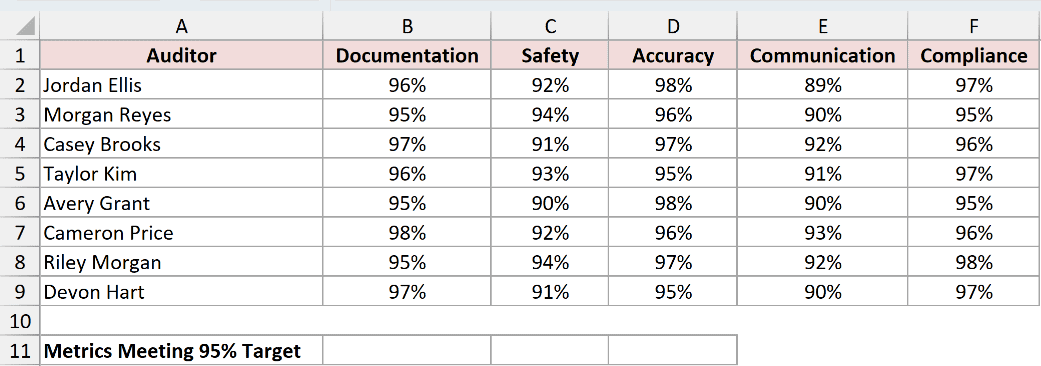
I want to return only the metric headers whose average score is at least 95%.

Here is the formula:

=FILTER(B1:F1,BYCOL(B2:F9,LAMBDA(c,AVERAGE(c)>=0.95)))

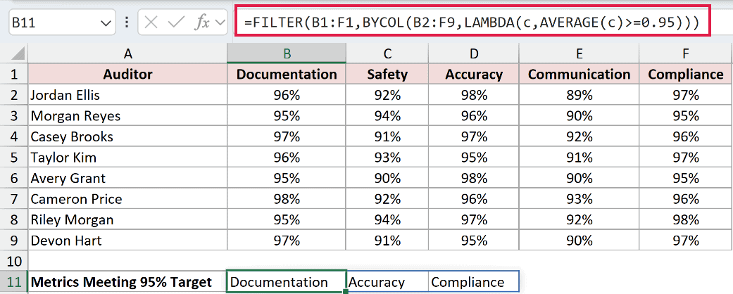
BYCOL returns one TRUE or FALSE for each metric, depending on whether its average reaches 95%.

FILTER uses that horizontal Boolean array to keep the matching headers. The result spills three names: Documentation, Accuracy, and Compliance.

Pro Tip: The header range and BYCOL result must have the same horizontal width. Here, both cover five metric columns.

Example 5: Stack High and Low Summaries

One formula can return more than one summary row.

Below is a renewal-rate table with seven cohorts across four months and a two-row summary area.

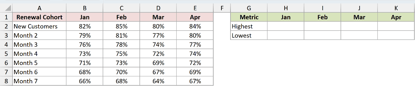
I want the highest and lowest renewal rates for every month.

Here is the formula:

=VSTACK(BYCOL(B2:E8,LAMBDA(c,MAX(c))),BYCOL(B2:E8,LAMBDA(c,MIN(c))))

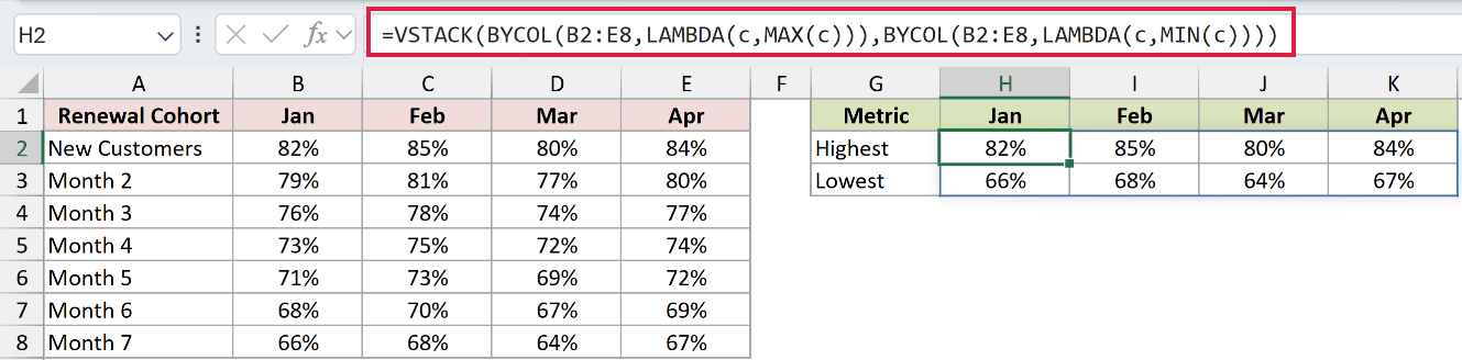
The first BYCOL returns the maximum for each month, and the second returns the minimum. VSTACK places the second result row below the first.

The highest rates are 82%, 85%, 80%, and 84%. The lowest rates are 66%, 68%, 64%, and 67%.

Pro Tip: Each LAMBDA must return one value per source column. Returning several values from one column produces a #CALC! error.

Tips & Common Mistakes

• BYCOL requires Microsoft 365 or Excel 2024. Excel 2021 and earlier return #NAME? because the function is unavailable.
• The LAMBDA must accept exactly one parameter. An invalid LAMBDA or wrong parameter count returns an Incorrect Parameters #VALUE! error.
• Use BYROW when each source row needs one result.
• Use MAP when you want to transform individual values rather than summarize whole columns.
• Dynamic array formulas cannot spill inside an Excel Table. Put the BYCOL formula in a normal worksheet range beside the table.
• Do not add @ before BYCOL. Implicit intersection would reduce the dynamic array behavior instead of returning the full horizontal result.

I covered column totals, conditional counts, filtered averages, header selection, and stacked high-and-low summaries with BYCOL.

I hope you found this article helpful.

List of All Excel Functions

Related Excel Functions / Articles:

• MAKEARRAY Function in Excel
• GROUPBY Function in Excel
• CHOOSECOLS Function in Excel