
Excel’s GROUPBY function groups records by one or more fields and returns an aggregated result for each group.
You can summarize sales by category or average values by department with a formula. The summary spills into nearby cells and can include totals, sorting, and filtering.
In this article, I’ll show you how to summarize expenses by department, group by multiple fields, and filter or sort the resulting summary.
GROUPBY Function Syntax in Excel
The GROUPBY function groups rows by one or more fields and calculates a summary for each group.
=GROUPBY(row_fields, values, function, [field_headers], [total_depth], [sort_order], [filter_array], [field_relationship])
- row_fields (required) contains the categories you want to group. You can supply one column or several adjacent columns.
- values (required) contains the numbers or other values you want to summarize.
- function (required) is the calculation to apply to each group, such as SUM, AVERAGE, PERCENTOF, or a custom LAMBDA.
- field_headers (optional) controls headers. Use 0 for none, 1 to hide existing headers, 2 to generate headers, or 3 to show existing headers.
- total_depth (optional) controls totals. Use 0 for none, 1 for a grand total, or 2 for a grand total and subtotals.
- sort_order (optional) identifies an output column to sort. A positive number sorts ascending, while a negative number sorts descending.
- filter_array (optional) supplies TRUE and FALSE values that decide which source rows GROUPBY includes.
- field_relationship (optional) uses 0 for hierarchical fields or 1 for independent table fields. Table mode does not support subtotals.
You can also use negative total_depth values. Use -1 for a grand total at the top or -2 for subtotals and a grand total at the top.
GROUPBY is available in Excel for Microsoft 365 on Windows, Mac, and the web. It is not available in Excel 2021 or Excel 2024 perpetual versions.
When to Use GROUPBY Function
- Summarize expenses, sales, hours, or quantities by a category.
- Build a report with several grouping levels and automatic subtotals.
- Sort grouped results by their labels or calculated values.
- Filter source rows before calculating each group’s result.
- Apply calculations such as SUM, AVERAGE, PERCENTOF, or a custom LAMBDA to every group.
Example 1: Total Expenses by Department
Let’s start with a basic summary of employee expense claims.
Below is the dataset. Columns A to C contain employees, departments, and claim amounts. Columns E and F will hold the grouped report.
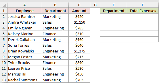
We want to calculate the total expenses for each department.
Here is the formula:
=GROUPBY(B2:B13,C2:C13,SUM)
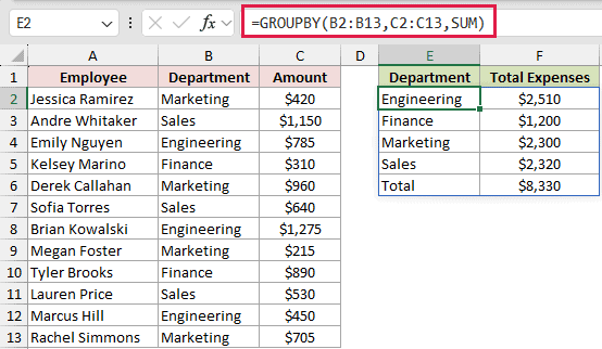
The range B2:B13 supplies the department names, while C2:C13 supplies the amounts. SUM tells GROUPBY how to combine each department’s claims.
The formula spills the summary into E2:F6. Engineering totals $2,510, Finance $1,200, Marketing $2,300, and Sales $2,320.
GROUPBY also adds a Total row of $8,330. Because no sorting option was supplied, the departments appear alphabetically.
Pro Tip: Keep the entire spill area empty. If any cell in E2:F6 already contains something, Excel returns #SPILL! instead of the grouped report.
Example 2: Average Attendance With Headers Shown
Now let’s calculate average attendance and let GROUPBY carry the source headers into the result.
Below is the dataset. Columns A to C list each class, instructor, and attendance count. The grouped result will begin in E1.
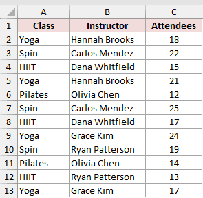
We want the average attendance for each class, with headers included in the spilled result.
Here is the formula:
=GROUPBY(A1:A13,C1:C13,AVERAGE,3)
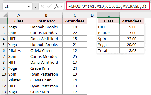
This time, both input ranges start in row 1 because they include their headers. The fourth argument, 3, tells GROUPBY to show those headers.
The result spills across E1:F6 with Class and Attendees at the top. HIIT averages 15 attendees, while Pilates, Spin, and Yoga average 13, 22, and 20.
The Total row returns the average across all 12 attendance records, which is 18.08.
Example 3: GROUPBY With Multiple Row Fields
Here’s how to build a two-level report with subtotals.
Below is the dataset. Columns A to C contain vehicle types, drivers, and fuel costs. Columns E to G will show the grouped results.
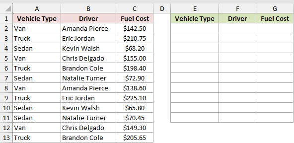
We want fuel costs grouped first by vehicle type and then by driver, with subtotals for each vehicle type.
Here is the formula:
=GROUPBY(A2:B13,C2:C13,SUM,0,2)
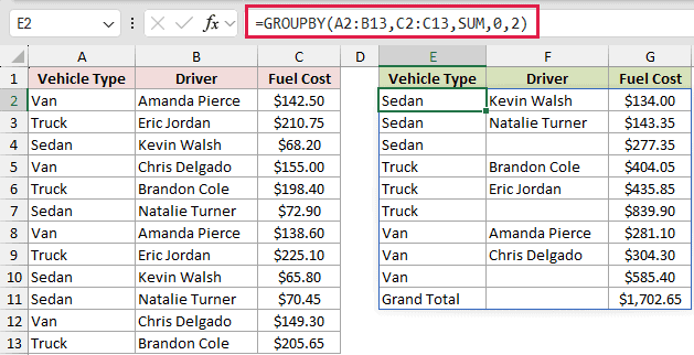
The row_fields argument covers two columns, so GROUPBY creates a hierarchy. Vehicle Type is the first level, and Driver is the second.
The fourth argument, 0, tells Excel that the selected ranges exclude headers. The fifth argument, 2, adds subtotals and a grand total.
Each subtotal row shows the vehicle type with a blank Driver cell, and the last row is labeled Grand Total.
Sedan costs total $277.35, Truck costs total $839.90, and Van costs total $585.40. The grand total is $1,702.65.
Pro Tip: Set field_relationship to 1 when grouping fields are independent columns instead of a hierarchy. Table mode does not support subtotals.
Example 4: Sort GROUPBY Results by Value
Next, we’ll rank cafe categories by weekly sales.
Below is the dataset. Columns A to C contain menu items, categories, and weekly sales. Columns E and F will contain the ranked summary.
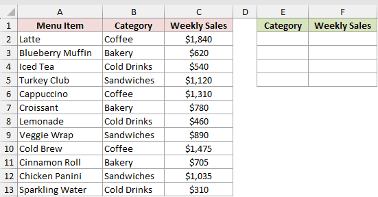
We want category totals sorted from the largest value to the smallest, without a Total row.
Here is the formula:
=GROUPBY(B2:B13,C2:C13,SUM,0,0,-2)
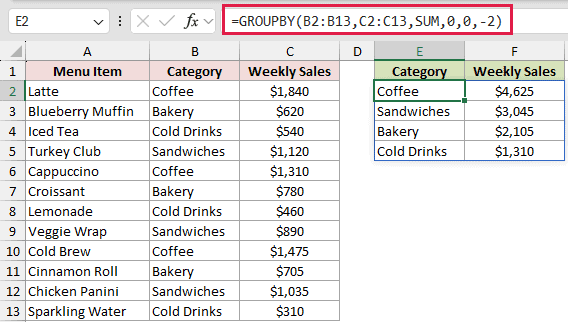
The fifth argument is 0, so GROUPBY leaves out the Total row. The sixth argument is -2, which sorts the second output column in descending order.
Coffee appears first with $4,625. Sandwiches follow at $3,045, then Bakery at $2,105 and Cold Drinks at $1,310.
You could build a separate SORTBY, UNIQUE, and SUMIFS formula for this report. GROUPBY handles the grouping and sorting in one formula.
Example 5: Filter Rows Before Grouping
Now let’s summarize only the tickets that meet a condition.
Below is the dataset. Columns A to D list ticket IDs, agents, priorities, and hours logged. The filtered summary will begin in F2.
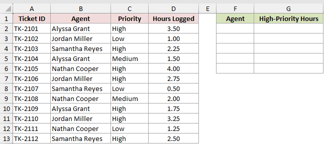
We want total hours by agent, but only for tickets marked High priority.
Here is the formula:
=GROUPBY(B2:B13,D2:D13,SUM,0,1,1,C2:C13="High")
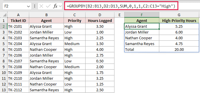
The filter_array argument tests whether each cell in C2:C13 equals High. GROUPBY ignores every source row where that test returns FALSE.
You could filter the source first with FILTER, but the filter_array argument keeps the condition inside the GROUPBY formula.
The fifth argument adds a grand total. The sixth argument sorts the first output column in ascending order, so the agents appear alphabetically.
Alyssa Grant has 5.25 hours, Jordan Miller 6.00, Nathan Cooper 4.00, and Samantha Reyes 4.75. The Total row returns 20.00 hours.
Pro Tip: The filter_array must have the same number of rows as row_fields. If the heights do not match, GROUPBY returns #VALUE!.
Example 6: Percent of Total and Custom LAMBDA
Finally, let’s use two different calculations on the same donation list.
Below is the dataset. Columns A to C contain donors, campaigns, and donation amounts. Two grouped reports will appear in columns E to I.
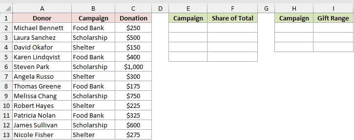
We want each campaign’s share of all donations and the difference between its largest and smallest gifts.
Here is the percentage formula:
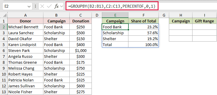
=GROUPBY(B2:B13,C2:C13,PERCENTOF,0,1)
And here is the custom LAMBDA formula:
=GROUPBY(B2:B13,C2:C13,LAMBDA(x,MAX(x)-MIN(x)),0,0)
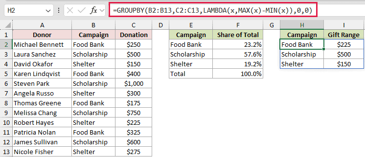
PERCENTOF divides each campaign’s total by the overall total. Food Bank receives 23.2%, Scholarship 57.6%, and Shelter 19.2%, followed by a 100% Total row.
The LAMBDA receives each campaign’s values as x, then subtracts the smallest gift from the largest. The resulting gift ranges are $225, $500, and $150.
Its fifth argument is 0, so the custom LAMBDA report does not include a Total row.
Pro Tip: PERCENTOF skips text cells in the values range. Only numeric values count toward each group’s share and the overall total.
Tips & Common Mistakes
- GROUPBY spills one report from a single formula. Clear enough room below and beside the formula before entering it.
- The
row_fields,values, andfilter_arrayranges must cover the same source rows. A missing or extra row causes an error or an incorrect grouping. - Positive
sort_ordervalues sort ascending. Negative values sort descending, and the number identifies the output column used for sorting. - Subtotals require at least two row fields in hierarchical mode. Setting
field_relationshipto 1 switches to table mode and removes subtotal support. - HSTACK can pass several functions to GROUPBY, such as SUM and PERCENTOF. Excel then adds an extra row above the spill containing the function names.
- If GROUPBY is unavailable in your Excel version, use a PivotTable or combine UNIQUE with SUMIFS, AVERAGEIFS, or another summary function.
I’ve shown you how to group rows, calculate totals and subtotals, sort results, and filter source data.
We also used PERCENTOF for shares of the total and a custom LAMBDA for calculations GROUPBY does not provide by itself.
Related Excel Functions / Articles:
