
The QUARTILE.EXC function in Excel returns an exclusive quartile from a numeric dataset. You can request the first quartile, median, or third quartile.
Unlike QUARTILE.INC, QUARTILE.EXC excludes the 0 and 1 percentile positions. That means it has no quart 0 or quart 4.
In this article, I’ll show you how exclusive ranks are interpolated, how EXC differs from INC, and how these quartiles can flag outliers.
QUARTILE.EXC Function Syntax in Excel
The function needs the numeric data and the quartile you want returned.
=QUARTILE.EXC(array, quart)
- array (required) is the range or array containing the numeric data.
- quart (required) selects Q1, the median, or Q3 by using 1, 2, or 3.
When to Use QUARTILE.EXC Function
- Find exclusive quartile cutoffs for a list of values.
- Compare exclusive and inclusive quartile conventions on the same data.
- Build outlier fences from exclusive quartiles.
- Calculate quartiles separately for filtered groups.
- Assign each record to a quartile group.
Example 1: Find First and Third Quartiles
A rent list makes the basic calculation easy to see.
Below is the dataset. Columns A and B list apartment units and monthly rents. The Q1 and Q3 cells wait in columns D and E.
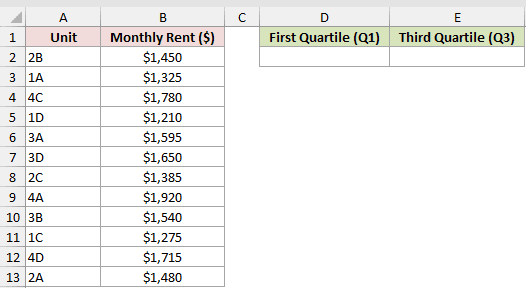
We want to calculate the first and third exclusive quartiles for the rent values.
Here is the Q1 formula:
=QUARTILE.EXC(B2:B13,1)
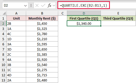
The formula returns $1,340.00 in D2.
And here is the Q3 formula:
=QUARTILE.EXC(B2:B13,3)
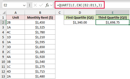
This formula returns $1,698.75 in E2.
QUARTILE.EXC sorts the numbers conceptually, so the worksheet data doesn’t need to be sorted first.
Excel calculates the exclusive rank as quart × (n + 1) / 4. With 12 rents, Q1 lands at 3.25 and Q3 at 9.75.
- At rank 3.25, Q1 sits one quarter of the way between $1,325 and $1,385, producing $1,340.00.
- At rank 9.75, Q3 sits three quarters of the way between $1,650 and $1,715, producing $1,698.75.
Example 2: Compare QUARTILE.EXC and QUARTILE.INC
The difference becomes clearer when both conventions use the same wait times.
Below is the dataset. Visit IDs and wait times occupy columns A and B. Column D contains quart inputs, with comparison results in columns E and F.
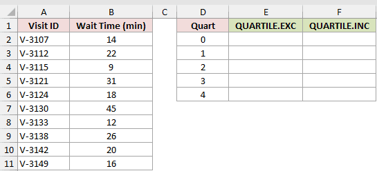
We want both functions to evaluate the same wait times for each quart value.
Here is the QUARTILE.EXC formula:
=QUARTILE.EXC($B$2:$B$11,D2:D6)
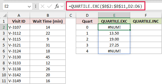
The formula spills results down column E. It returns 13.50, 19.00, and 27.25 for quart values 1, 2, and 3.
The cells for quart 0 and quart 4 deliberately return #NUM!. QUARTILE.EXC has no quart code for the minimum or maximum.
With exactly 3 values, though, Q1 and Q3 can still equal the minimum and maximum, as Example 4 shows.
And here is the QUARTILE.INC formula for comparison:
=QUARTILE.INC($B$2:$B$11,D2:D6)
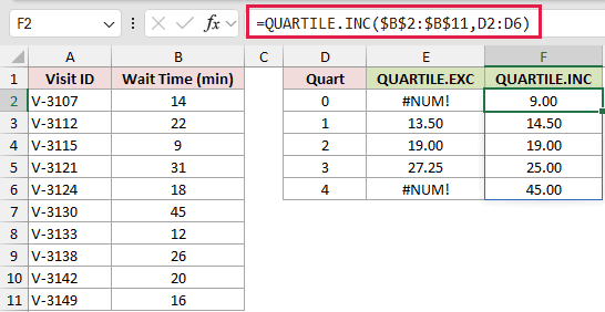
QUARTILE.INC returns 9.00, 14.50, 19.00, 25.00, and 45.00. The median matches, but the first and third quartiles differ.
Range-based spills work in Excel 2021, Excel 2024, and Microsoft 365.
Pro Tip: On the same wait times, EXC gives Q1 as 13.50 and Q3 as 27.25, compared with 14.50 and 25.00 from INC. Name the convention when sharing cutoffs.
Example 3: Flag Outliers With EXC Fences
Here’s a practical way to identify unusually fast or slow payments.
Below is the dataset. Columns A and B list customers and days to pay. Column C will hold flags, while the labeled cells in E:F build the fence calculations.
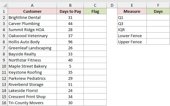
We want to calculate the exclusive quartiles, build the lower and upper fences, then flag values outside them.
First, calculate Q1:
=QUARTILE.EXC(B2:B16,1)
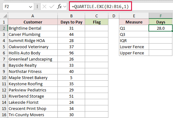
Q1 is 28.0 days.
Next, calculate Q3:
=QUARTILE.EXC(B2:B16,3)
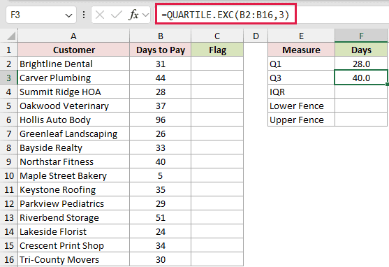
Q3 is 40.0 days.
Subtract Q1 from Q3 to get the IQR, or interquartile range:
=F3-F2
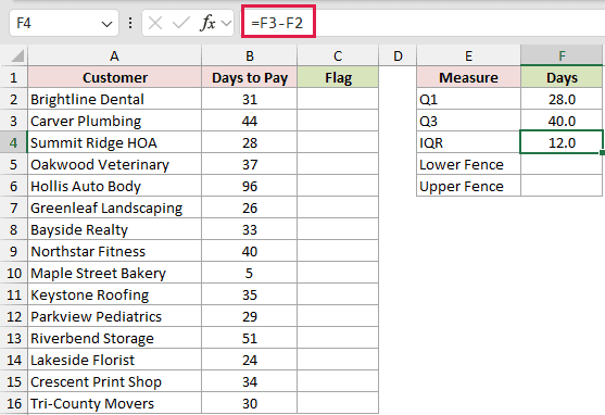
The IQR is 12.0 days.
The standard fence rule extends 1.5 times the IQR below Q1 and above Q3.
Here is the lower-fence formula:
=F2-1.5*F4
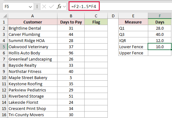
The lower fence is 10.0 days.
And here is the upper-fence formula:
=F3+1.5*F4
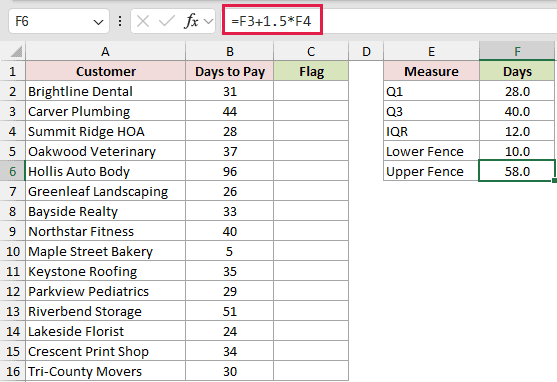
The upper fence is 58.0 days.
Finally, use those fences to label every customer:
=IF((B2:B16<F5)+(B2:B16>F6),"Outlier","OK")
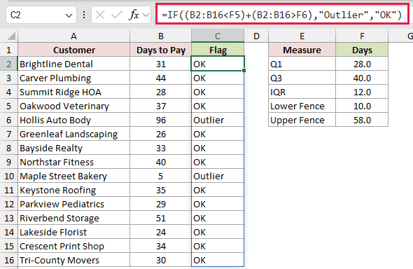
The formula spills down column C. Hollis Auto Body at 96 days and Maple Street Bakery at 5 days are labeled Outlier.
The + adds the two TRUE/FALSE tests for each row. If either test returns TRUE, the sum is 1 and IF labels that row Outlier.
Using OR on the range tests would collapse them into one TRUE or FALSE result.
Example 4: Calculate Quartiles by Department
Department-level hiring data shows how the same calculation works with filtered groups.
Below is the dataset. Columns A:C list openings, departments, and days to fill. The E:I panel will show group counts and three quartile results.
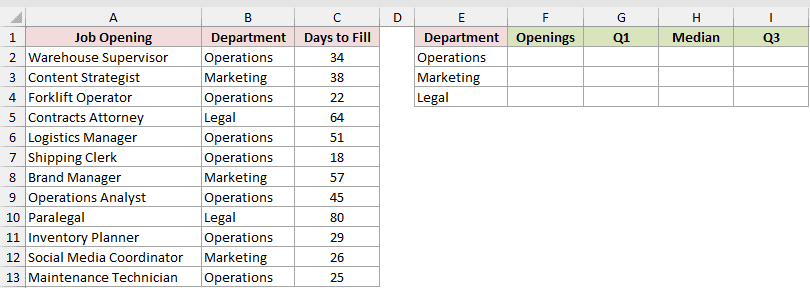
We want to count each department’s openings, filter its hiring times, and return Q1, the median, and Q3.
First, count the openings for the department in E2:
=COUNTIF($B$2:$B$13,E2)
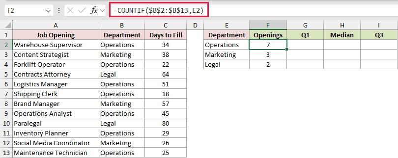
Copying the formula down returns 7 for Operations, 3 for Marketing, and 2 for Legal.
Here is the Operations quartile formula:
=QUARTILE.EXC(FILTER($C$2:$C$13,$B$2:$B$13=$E2),{1,2,3})
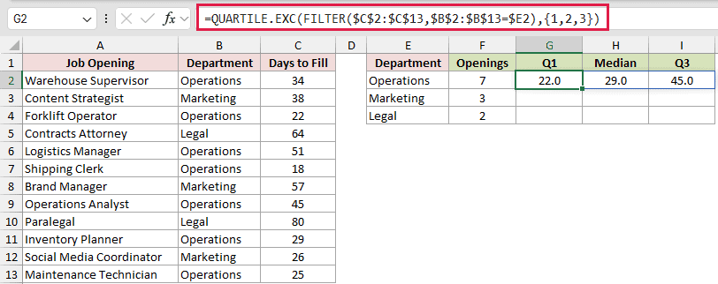
FILTER passes only Operations values to QUARTILE.EXC. The formula spills 22.0, 29.0, and 45.0 across G2:I2.
Here is the Marketing quartile formula:
=QUARTILE.EXC(FILTER($C$2:$C$13,$B$2:$B$13=$E3),{1,2,3})
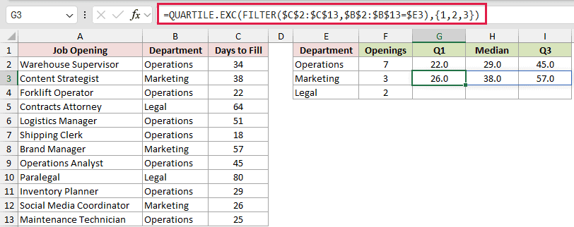
Marketing has 3 values, so the formula returns 26.0, 38.0, and 57.0.
And here is the Legal quartile formula:
=QUARTILE.EXC(FILTER($C$2:$C$13,$B$2:$B$13=$E4),{1,2,3})
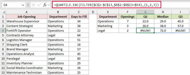
Legal has 2 values. Its median is 72.0, while Q1 and Q3 deliberately return #NUM! because those quartiles need at least 3 values.
FILTER and these spilled results require Excel 2021 or later.
Example 5: Assign Each Row a Quartile Group
The same cutoffs can also label each branch.
Below is the dataset. Columns A and B contain branches and funded loans. Each branch’s quartile group will appear in column C.
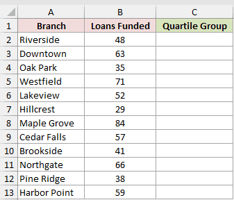
We want to compare every branch with all three exclusive quartile cutoffs and return a group number.
Here is the first-row formula:
=1+SUM(--(B2>QUARTILE.EXC($B$2:$B$13,{1,2,3})))
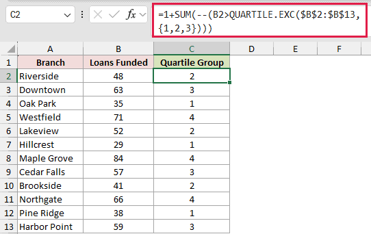
Copy the formula down column C. It returns group 2 for Riverside, group 1 for Hillcrest, and group 4 for Maple Grove.
Group 1 is the bottom quarter, and group 4 is the top quarter. Because the test uses >, a value equal to a cutoff stays in the lower group.
QUARTILE.EXC returns the three cutoffs inside the formula. Each TRUE comparison becomes 1, SUM counts the passed cutoffs, and the leading 1 sets the group.
Tips & Common Mistakes
- QUARTILE.EXC accepts quart values 1, 2, and 3. Quart 0 and quart 4 return #NUM!, so use MIN or MAX when you need an endpoint.
- A decimal quart is truncated. In testing, quart 1.7 behaves like quart 1.
- A quart stored as the text “1” works, but nonnumeric text such as “abc” returns #VALUE!.
- Text and TRUE values inside the data range are ignored, but an #N/A value propagates.
=AGGREGATE(19,6,range,1)skips errors and returns the same Q1 as error-free data. - QUARTILE.EXC normally reduces a data range to one result, but a quart range or array can spill several results.
QUARTILE.EXC turns a numeric range into exclusive Q1, median, and Q3 cutoffs.
The same cutoffs can feed outlier fences, filtered summaries, and row-level group labels.
Related Excel Functions / Articles:
