QUARTILE.INC Function in Excel

If you have a list of numbers and want to know how the values are spread out, the QUARTILE.INC function gives you a quick way to split your data into four equal parts.

In this article, I’ll show you how QUARTILE.INC works and walk through five practical examples that cover the most common things people actually use it for.

QUARTILE.INC Function Syntax

Here is the syntax of the QUARTILE.INC function:

=QUARTILE.INC(array, quart)

• array – The range or array of numeric values you want to analyze.
• quart – A number from 0 to 4 that tells Excel which quartile to return. 0 is the minimum, 1 is the first quartile (Q1), 2 is the median, 3 is the third quartile (Q3), and 4 is the maximum.

QUARTILE.INC was added in Excel 2010 and replaces the older QUARTILE function with the same behavior. If you’re on a recent version, use QUARTILE.INC.

When to Use the QUARTILE.INC Function

Use this function when you need to:

• Find the 25th, 50th, or 75th percentile of a dataset
• Identify the top or bottom 25% of values in a list
• Calculate the interquartile range (IQR) for outlier detection
• Compare how a single value sits within a larger group
• Build box plot inputs without manually sorting the data

Let me show you a few practical examples of how to use this function.

Example 1: Find the First and Third Quartiles

Let’s start with a simple example.

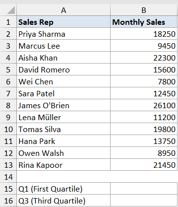
Below is the dataset. It has the monthly sales figures for 12 sales reps in a small team. Column A has the rep names and column B has each rep’s total sales for the month.

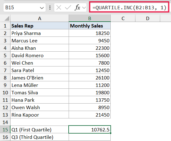
I want to find the first quartile (Q1) and the third quartile (Q3) of the sales figures so I can see the cut-off for the bottom 25% and top 25% of the team.

Here is the formula for Q1:

=QUARTILE.INC(B2:B13, 1)

And here is the formula for Q3:

=QUARTILE.INC(B2:B13, 3)

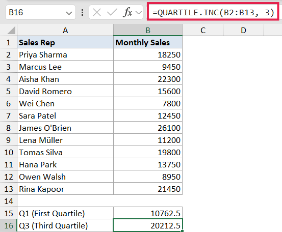
In the above formulas, B2:B13 is the range of sales figures. The second argument tells QUARTILE.INC which quartile to return. Pass 1 for the first quartile and 3 for the third quartile.

Any rep with sales at or below the Q1 value sits in the bottom quarter of the team. Any rep at or above Q3 sits in the top quarter.

Example 2: Return All Five Quartile Values at Once

Here’s a slightly more interesting scenario.

Below is the same dataset. This time I want all five quartile breakpoints (min, Q1, median, Q3, max) listed in one go, rather than typing five separate formulas.

I want one formula that returns the full quartile breakdown in a vertical list.

Here is the formula:

=QUARTILE.INC(B2:B13, SEQUENCE(5, 1, 0, 1))

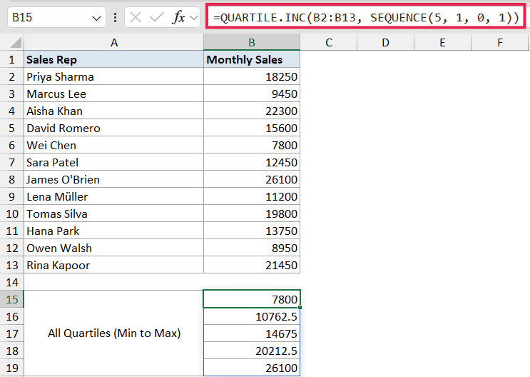
How this formula works:

• SEQUENCE(5, 1, 0, 1) builds the array {0; 1; 2; 3; 4}, one row each.
• That array gets fed in as the quart argument.
• QUARTILE.INC runs once for each value in the sequence and spills the five results into the cells below.

This is one of the few cases where a function that normally returns a single value still produces a spill. The spill comes from the SEQUENCE side, not from QUARTILE.INC itself.

If you’re on Excel 2019 or earlier, SEQUENCE isn’t available. In that case, type the five formulas separately (=QUARTILE.INC(B2:B13, 0), =QUARTILE.INC(B2:B13, 1), and so on) in five cells.

Example 3: Calculate the Interquartile Range (IQR)

Now let’s look at something you’ll see in almost every stats course.

Below is a dataset of customer order values from an online store. Column A has the order ID and column B has the order amount in dollars.

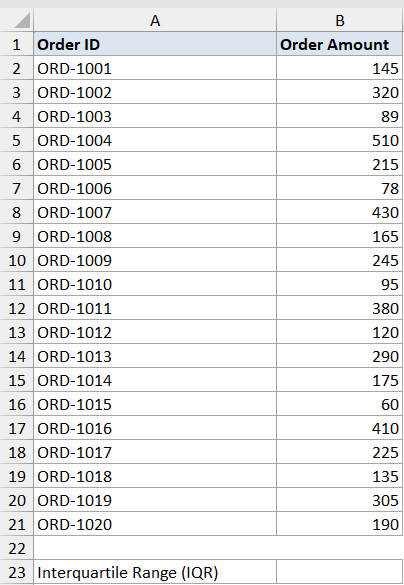
I want to calculate the interquartile range, which is Q3 minus Q1. The IQR tells me the spread of the middle 50% of my orders, which is a more stable measure than the full range when there are a few very large orders.

Here is the formula:

=QUARTILE.INC(B2:B21, 3) - QUARTILE.INC(B2:B21, 1)

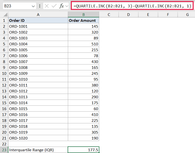
In the above formula, the first QUARTILE.INC returns the third quartile of the order amounts, and the second one returns the first quartile. Subtract them and you get the IQR.

A wider IQR means orders vary a lot in the middle of the distribution. A narrower IQR means most of your middle orders cluster tightly around the median.

Example 4: Flag Outliers Using the 1.5*IQR Rule

This is the example most people actually came here for.

Below is a dataset of delivery times (in hours) for a logistics team across 18 shipments. Column A has the shipment ID and column B has the delivery time.

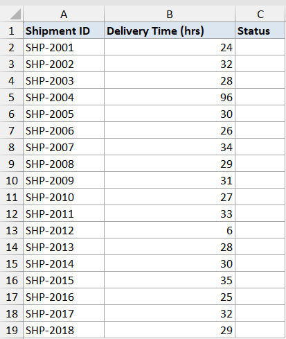
I want to flag any shipment whose delivery time is unusually long or short using the standard 1.5*IQR rule. An outlier is anything below Q1 - 1.5*IQR or above Q3 + 1.5*IQR.

Here is the formula in the helper column (entered in C2 and filled down):

=IF(OR(B2<QUARTILE.INC($B$2:$B$19,1)-1.5*(QUARTILE.INC($B$2:$B$19,3)-QUARTILE.INC($B$2:$B$19,1)), B2>QUARTILE.INC($B$2:$B$19,3)+1.5*(QUARTILE.INC($B$2:$B$19,3)-QUARTILE.INC($B$2:$B$19,1))), "Outlier", "Normal")

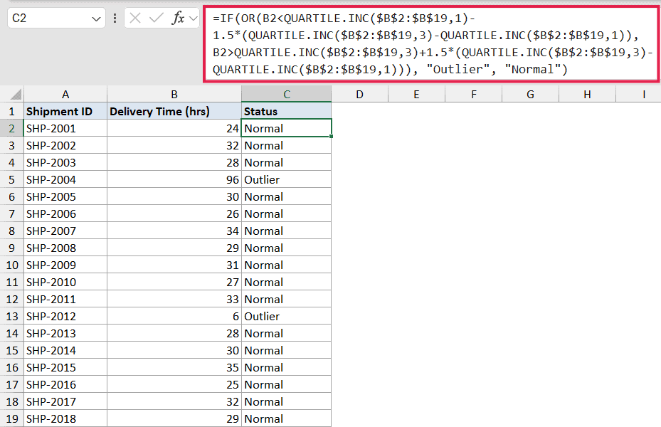
How this formula works:

• The inner QUARTILE.INC($B$2:$B$19,1) and QUARTILE.INC($B$2:$B$19,3) return Q1 and Q3 for the full delivery-time column.
• (Q3 - Q1) * 1.5 is the IQR multiplied by 1.5.
• Q1 minus that value is the lower fence; Q3 plus that value is the upper fence.
• The IF checks whether the row’s delivery time falls outside either fence, and labels it “Outlier” or “Normal”.

For a cleaner version, put Q1 and Q3 in two helper cells (say, E1 and E2), then reference them in the IF. The formula gets much shorter and the QUARTILE.INC functions only have to evaluate twice instead of four times per row.

We’re keeping this as a per-row formula because we need a per-shipment label. In 365 you can also write it as a single spilling array formula, but you have to swap the OR for boolean math (OR collapses an array to one value), e.g. =IF((B2:B19<Q1-1.5*IQR)+(B2:B19>Q3+1.5*IQR), "Outlier", "Normal").

Example 5: Quartile for a Filtered Subset

Let’s step it up with a more advanced use case.

Below is a dataset of employee salaries across multiple departments. Column A has the employee name, column B has the department, and column C has the annual salary.

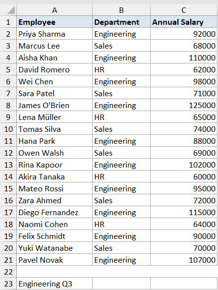
I want the third quartile of salaries, but only for employees in the “Engineering” department. The plain QUARTILE.INC reads the whole column, so I need to feed it just the filtered values.

Here is the formula:

=QUARTILE.INC(FILTER(C2:C21, B2:B21="Engineering"), 3)

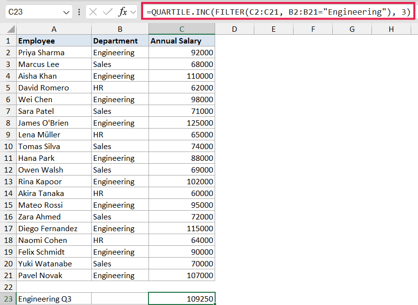
In the above formula, FILTER returns just the salary values where the department matches “Engineering”. QUARTILE.INC then computes the third quartile on that smaller array.

This is a clean way to get a conditional quartile without building helper columns. Swap the department name to get the Q3 for another team, or wrap the whole formula in a SEQUENCE-driven spill to get all five quartiles for the filtered subset at once.

If you’re on an older version of Excel that doesn’t have FILTER, you can use an array formula with IF: =QUARTILE.INC(IF(B2:B21="Engineering", C2:C21), 3) entered with Ctrl+Shift+Enter.

Tips & Common Mistakes

• QUARTILE.INC vs QUARTILE.EXC: QUARTILE.INC includes the minimum and maximum values when computing quartiles. QUARTILE.EXC excludes them and cannot return a value for quart=0 or quart=4. INC is the more common choice for general business analysis. EXC tends to come up in academic statistics.
• Quart must be between 0 and 4: If you pass any other number, QUARTILE.INC returns a #NUM! error. Decimals get truncated, so 1.9 is treated as 1.
• Empty range returns #NUM!: If the array is empty or contains only text, you’ll get a #NUM! error. Wrap the function in IFERROR if your dataset can be empty.
• Text and blank values are ignored: QUARTILE.INC skips blanks, text, and logical values inside the range. It only operates on numbers. This is usually what you want, but worth noting if you expect specific behavior with mixed data.
• QUARTILE is the legacy version: The older QUARTILE function still works for backward compatibility, but Microsoft recommends QUARTILE.INC for any file used in Excel 2010 or later. They behave identically.
• Related function for arbitrary percentiles: If you need a percentile that isn’t 25, 50, or 75 (say, the 90th percentile), use PERCENTILE.INC instead. QUARTILE.INC is just a shortcut for the four standard quartile percentiles.

QUARTILE.INC is one of those functions that looks niche but turns out to be useful in a lot of everyday spreadsheets, from sales analysis to outlier detection to grading curves.

The syntax is straightforward and once you know how the quart argument works, you can pull any of the five breakpoints in a single formula.

If you find yourself reaching for QUARTILE.INC often, learning PERCENTILE.INC and the FILTER function will multiply what you can do with it.

List of All Excel Functions