
Excel’s IMABS function returns the absolute value, or modulus, of a complex number as a real number.
The result is always nonnegative. Because it is numeric, it can feed ordinary arithmetic, sorting, or comparisons.
In this article, I’ll show you how to turn complex-number text into a magnitude, calculate electrical current from impedance, and spot invalid input formats.
IMABS Function Syntax in Excel
The IMABS function accepts complex-number text or a plain real number.
=IMABS(inumber)
- inumber (required) is the value whose absolute value you want. It can be complex-number text in x+yi or x+yj form, using lowercase i or j, or a plain real number.
When entering a complex literal directly in the formula, put it in quotation marks.
When to Use IMABS Function
- Find the magnitude of a complex number stored in a cell.
- Calculate electrical current from voltage and complex impedance.
- Measure the distance between target and measured complex coordinates.
- Rank complex values by magnitude instead of sorting their text.
Example 1: Calculate a Complex Number’s Magnitude
Let’s start with several complex numbers that use positive and negative parts.
Below is the dataset. Column A contains the complex numbers, while the green header and empty cells in column B show where their absolute values will appear.
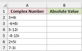
Column B should return the magnitude of each complex number.
Here is the formula entered in B2 and copied down the column:
=IMABS(A2)
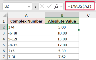
The formula returns 5.00 for 3+4i and 17.00 for -8-15i. Negative real or imaginary parts do not make the magnitude negative.
Geometrically, IMABS measures the distance from zero to the complex number on the complex plane.
Example 2: Calculate Electrical Current From Impedance
Here’s an electrical example that uses impedance written with j.
Below is the dataset. It lists equipment, supply voltage, and impedance. The green columns will hold impedance magnitude and calculated current.
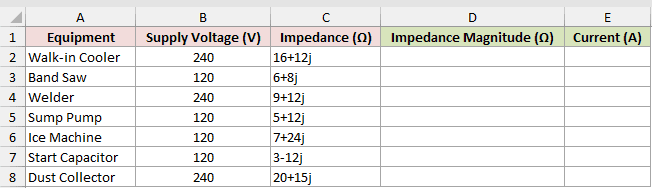
The first step is finding a numeric magnitude for each impedance.
Here is the formula entered in D2 and copied down:
=IMABS(C2)
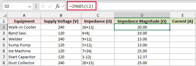
The Walk-in Cooler’s 16+12j impedance has a magnitude of 20.00. The Band Saw’s 6+8j impedance has a magnitude of 10.00.
We can now use that numeric result to calculate current in column E.
Here is the formula entered in E2 and copied down:
=B2/D2
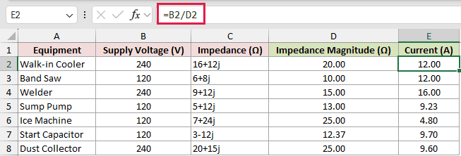
The Walk-in Cooler and Band Saw both return 12.00 amps. Their voltages and impedance magnitudes differ, but the division produces the same current.
Example 3: Measure Complex Coordinate Position Error
Suppose you need to measure how far each drilled hole is from its target position.
Below is the dataset. It pairs each target and measured complex coordinate, with a green position-error column waiting for the calculated distance.
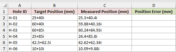
For each hole, the required result is the distance between its measured position and target.
Here is the formula entered in D2 and copied down:
=IMABS(IMSUB(C2,B2))
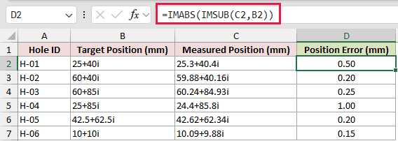
IMSUB calculates the complex difference between the measured and target positions. IMABS then converts that difference into a real, nonnegative distance.
H-01 has a position error of 0.50 mm. H-04 stands out at 1.00 mm, while H-06 returns 0.15 mm.
Reversing the IMSUB arguments changes the direction of the difference, but its magnitude stays the same.
Example 4: Compare IMABS With Its Expanded Calculation
To check the calculation, we’ll rebuild each phasor’s magnitude from its parts.
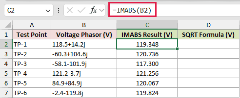
Below is the dataset. Column B contains voltage phasors. Columns C and D will hold the IMABS result and the calculation rebuilt from the real and imaginary parts.
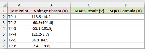
Column C should return the magnitude directly with IMABS.
Here is the formula entered in C2 and copied down:
=IMABS(B2)
Next, column D will calculate the same magnitude from the real and imaginary parts.
Here is the comparison formula entered in D2 and copied down:
=SQRT(IMREAL(B2)^2+IMAGINARY(B2)^2)
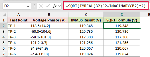
The comparison squares the real and imaginary parts, adds them, and returns the square root. IMABS handles those steps in one function.
Both formulas return 119.348 for TP-1 and 121.256 for TP-4. Every displayed result in the two columns matches.
If the parts already sit in separate cells, =IMABS(COMPLEX(6,8)) returns 10, so you do not need to assemble the complex-number text first.
Example 5: Sort Complex Numbers by Magnitude
A spilled formula can rank the entire list at once.
Below is the dataset. Columns A and B hold feeder names and fault-current text. Columns D and E are reserved for the ranked table.
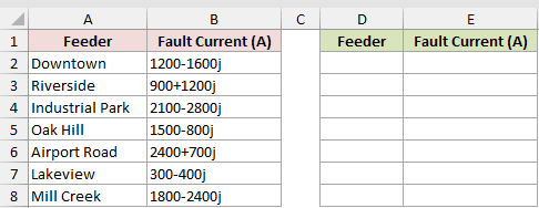
Enter one formula in D2 to sort the feeders from largest to smallest magnitude. The ranked table will spill through D2:E8.
Here is the formula:
=SORTBY(A2:B8,IMABS(B2:B8&""),-1)
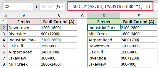
SORTBY returns the source rows in magnitude order. Industrial Park appears first with 2100-2800j, while Lakeview appears last with 300-400j.
The &"" converts B2:B8 into a calculated text array. That lets IMABS evaluate every entry as the hidden sort key.
A plain range passed to IMABS returns one #VALUE! instead of spilling. The coercion in this formula avoids that range behavior.
This spill works in Excel 2021, Excel 2024, and Microsoft 365. The returned table keeps the original feeder names and complex values.
In versions without dynamic-array spills, fill down an IMABS helper column and sort the table normally.
Pro Tip: Keep the output area in columns D and E empty so the sorted table has room to spill.
Example 6: Handle Different IMABS Input Forms
The last example tests several valid input forms and one deliberate error.
Below is the dataset. Column B contains complex and real inputs. The green result column will show the absolute value or the intended error.
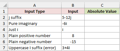
The result column should show the absolute value or the intended error for each input.
Here is the formula entered in C2 and copied down:
=IMABS(B2)
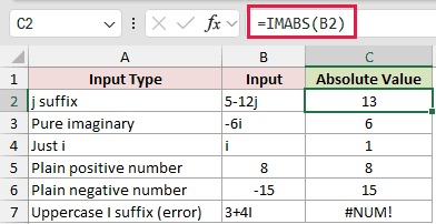
The j-suffix value 5-12j returns 13. The pure imaginary value -6i returns 6, and i by itself returns 1.
Plain numeric inputs work too. The positive input returns 8, while -15 returns 15.
The final row deliberately uses uppercase I. Excel returns #NUM!, so use a lowercase i or j suffix in complex-number text.
Tips & Common Mistakes
- Both lowercase i and lowercase j are valid suffixes. Uppercase I returns #NUM!.
- Plain positive and negative numbers are accepted. IMABS returns their ordinary absolute values.
- Keep the real part before the imaginary part. Inputs such as
3+j4and4i+3return#NUM!. - Placeholder text such as
TBDand an empty string""return#NUM!. This does not describe a truly blank cell. - Excel accepts the unusual text
3+-7i, and IMABS returns7.615773.
IMABS is most useful when a complex value must participate in a calculation that expects an ordinary number.
That numeric magnitude is the bridge between Excel’s complex-number text and the rest of your worksheet.
Other Excel articles you may also like:
