
Excel’s TANH function returns the hyperbolic tangent of any real number as a value between -1 and 1.
Its S-shaped curve keeps zero at zero, preserves the input’s sign, and reduces the influence of very large positive or negative values.
In this article, I’ll show you how to build trend scores, model an S-curve rollout, and calculate correlation confidence limits.
TANH Function Syntax in Excel
The TANH function needs one number and returns its hyperbolic tangent.
=TANH(number)
- number (required) is any real number for which you want the hyperbolic tangent.
When to Use TANH Function
- Compress an unbounded signed metric into a score near -1 to 1.
- Model an S-shaped increase that starts slowly, rises quickly, and then levels off.
- Apply a zero-centered activation to a weighted sum.
- Convert Fisher z values back to correlation coefficients.
- Avoid overflow problems in expanded formulas built with EXP.
Example 1: See TANH Across a Number Range
Let’s start by seeing how TANH behaves across negative and positive inputs.
Below is the dataset. Column A contains nine input numbers. The green TANH Result header and empty cells in column B mark the spilled output range.
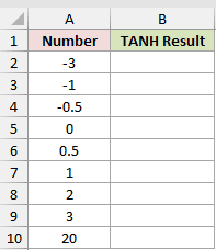
We want one formula in B2 to return the TANH result for every number.
Here is the formula:
=TANH(A2:A10)
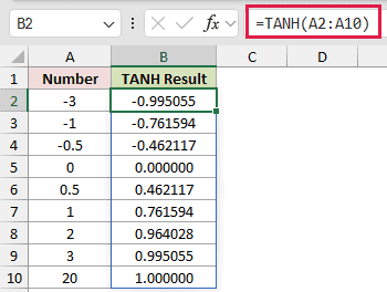
The formula returns -0.995055 for -3, zero for 0, and 0.995055 for 3. The mirrored signs show TANH’s odd symmetry.
At 20, Excel displays 1.000000 because TANH is already extremely close to its upper limit.
This range formula spills in Excel 2021, Excel 2024, and Microsoft 365. Excel 2019 and earlier need a formula in each row.
Example 2: Scale Sales Changes Into Trend Scores
Here’s a practical way to keep one unusual change from dominating a comparison.
Below is the dataset. It lists each Store and its Sales Change vs Last Year. The green Trend Score column contains empty result cells.
The Scale card in column E holds 10%, which controls how quickly the scores flatten.
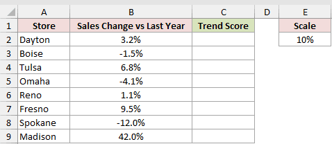
We want to convert every sales change into a signed score using that 10% scale.
Here is the formula:
=TANH(B2:B9/$E$2)
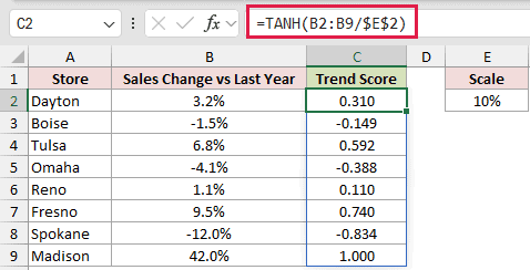
Dayton’s 3.2% change returns 0.310, while Spokane’s -12.0% returns -0.834. Madison’s 42.0% displays 1.000 instead of dominating the scale.
The sign still shows direction. Dividing by the scale controls how quickly larger changes move toward -1 or 1.
Pro Tip: Increase the Scale value in $E$2 for gentler compression, or reduce it when you want scores to flatten sooner.
Example 3: Model an S-Curve Rollout
Now let’s turn TANH into a gradual adoption curve over time.
Below is the dataset. Column A lists weeks 1 through 12, and the green Employees Using the Tool column waits for results.
The Setting and Value card contains Total Employees, Midpoint Week, and Ramp Width (Weeks), with values 480, 6, and 2.
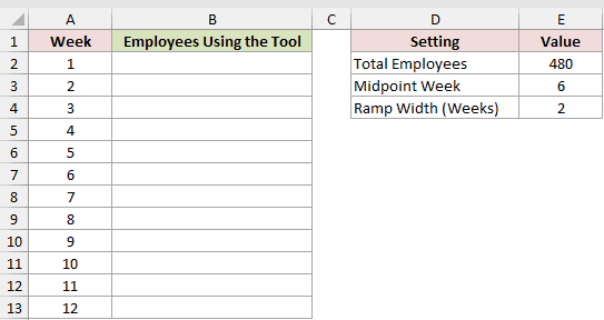
We want to estimate how many employees are using the tool during each week.
Here is the formula:
=$E$2*(1+TANH((A2:A13-$E$3)/$E$4))/2
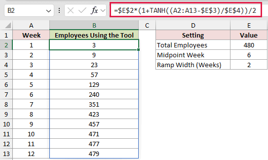
The result rises from 3 employees in week 1 to 240 in week 6, then reaches 479 by week 12.
Week 6 returns half of the 480-employee total because the adjusted TANH input is zero at the midpoint.
Charting Week against the spilled Employees Using the Tool results will show the S-shaped rollout clearly.
Example 4: Apply TANH as an Activation Function
This example applies TANH to a weighted lead score.
Below is the dataset. Each Lead has Email Opens, Pages Viewed, and a Demo Requested value of 1 or 0.
The green Weighted Sum and TANH Activation columns contain empty result cells.
The Input and Weight card assigns weights of 0.3, 0.2, and 1.5, plus a Bias of -2.5.
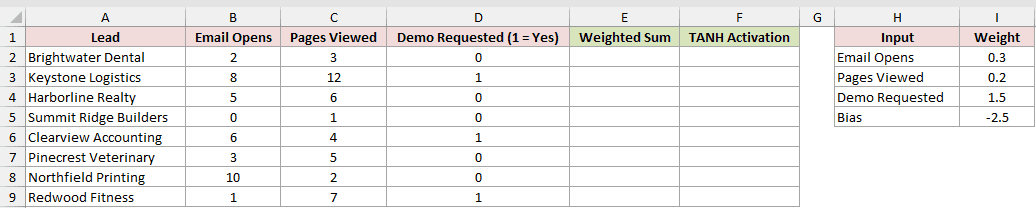
First, we want to calculate the weighted sum for every lead.
Here is the formula:
=B2:B9*$I$2+C2:C9*$I$3+D2:D9*$I$4+$I$5
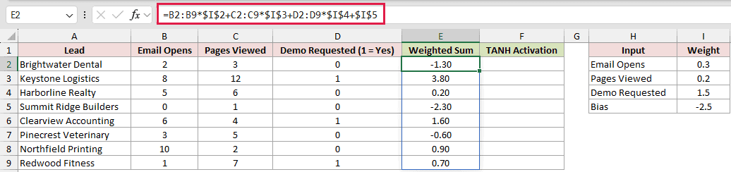
Next, TANH will compress those weighted sums into activation values.
Here is the formula:
=TANH(E2:E9)
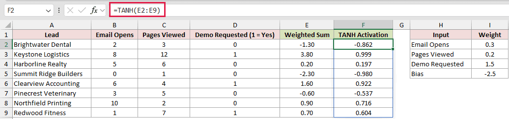
Brightwater Dental has a weighted sum of -1.30 and an activation of -0.862. Keystone Logistics has 3.80 and an activation of 0.999.
In this model, a positive activation leans toward conversion, while a negative activation points the other way.
Example 5: Calculate Correlation Confidence Limits
Here’s a statistical use that pairs TANH with its inverse, ATANH.
Below is the dataset. Columns A through C list six relationships, their correlations, and sample sizes.
The two answer areas are empty bordered cells under the green Lower 95% Limit and Upper 95% Limit headers.
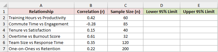
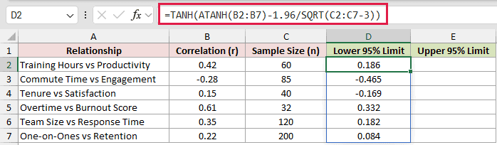
We want to calculate the lower confidence limit for every correlation first.
Here is the formula:
=TANH(ATANH(B2:B7)-1.96/SQRT(C2:C7-3))
The upper-limit formula adds the same margin in Fisher z space.
Here is the formula:
=TANH(ATANH(B2:B7)+1.96/SQRT(C2:C7-3))
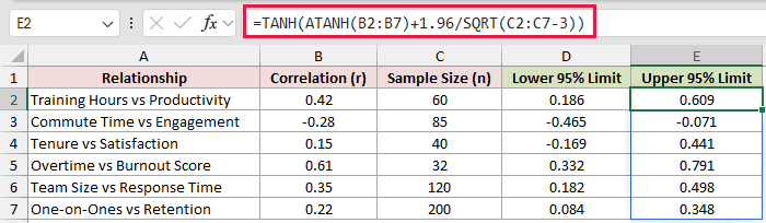
ATANH first moves each correlation into Fisher z space. The term 1.96/SQRT(n-3) supplies the 95% margin before TANH converts the limits back.
For Training Hours vs Productivity, the interval runs from 0.186 to 0.609 around a correlation of 0.42.
The two limits don’t have to sit the same distance from the original correlation, but both stay inside -1 and 1.
Pro Tip: You can replace the rounded 1.96 constant with NORM.S.INV(0.975), which returns 1.959964.
Example 6: Compare TANH With the EXP Formula
Finally, let’s compare TANH with an expanded version built from EXP.
Below is the dataset. Column A contains seven numbers. The green TANH Result and EXP Formula Result columns contain empty cells for the two calculations.
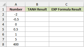
First, we want the built-in TANH result for each number.
Here is the formula:
=TANH(A2:A8)
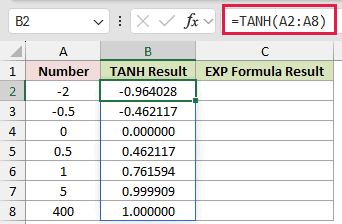
Now we’ll calculate the same values with the equivalent EXP expression.
Here is the comparison formula:
=(EXP(2*A2:A8)-1)/(EXP(2*A2:A8)+1)
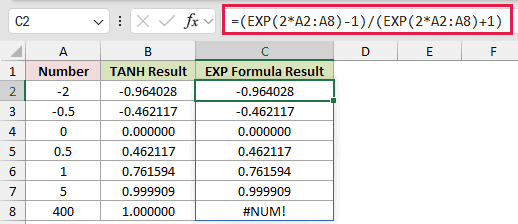
The displayed results match from -2 through 5, including 0.999909 at an input of 5.
At 400, TANH returns 1 and displays it as 1.000000. The expanded expression tries to calculate EXP(800), so Excel returns #NUM! instead.
The built-in function is shorter and handles this extreme input without that overflow error.
Tips & Common Mistakes
- TANH works with real numbers, not circular angles. Don’t convert degrees with RADIANS or multiply by PI()/180 before using it.
- A blank cell is treated as zero. A cell containing TRUE is treated as 1 and returns 0.761594.
- Text such as
abcand an empty text string""return#VALUE!. - Keep the spill area empty in Excel 2021, Excel 2024, and Microsoft 365. A blocked output range returns
#SPILL!. - The
@operator before TANH collapses a range calculation to one cell instead of returning the full spilled array. - ATANH is the inverse function, but its input must be strictly between -1 and 1.
- TANH is zero-centered from -1 to 1. A sigmoid is a better fit when the required output range is 0 to 1.
Choose a Scale divisor that matches your data.
For an S-curve rollout, adjust the Midpoint and Ramp Width settings until the curve matches the pace you expect.
Related Excel Functions / Articles:
