
Excel’s MODE.SNGL function returns the most frequently occurring number in a set of values.
When several numbers share the highest frequency, it returns whichever tied value appears first in the data. If no number repeats, it returns #N/A.
In this article, I’ll show you how to find modes by category, handle ties and missing repeats, work with text, and compare mode with median and average.
MODE.SNGL Function Syntax in Excel
The MODE.SNGL function accepts numbers, cell references, ranges, or arrays.
=MODE.SNGL(number1,[number2],...)
- number1 (required) is the first number, reference, range, or array you want to evaluate.
- number2, … (optional) adds more numbers, references, ranges, or arrays, with up to 254 number arguments in total.
When to Use MODE.SNGL Function
- Find the most common size, score, quantity, or rating in a list.
- Calculate a separate mode for each product, team, region, or other category.
- Compare the mode with the median and average when unusual values skew the data.
- Return one tied mode when you only need a single answer.
- Find the most common value in each row of a table.
Example 1: Find the Most Common Shoe Size
Let’s start with a simple retail example.
Below is the dataset. It lists receipt numbers and shoe sizes, followed by labeled empty cells for the most common size and its sales count.
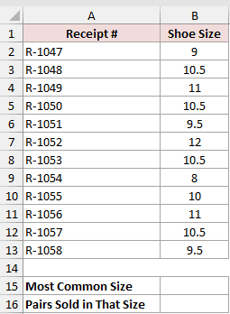
We want to identify the most common shoe size and count how many pairs were sold in that size.
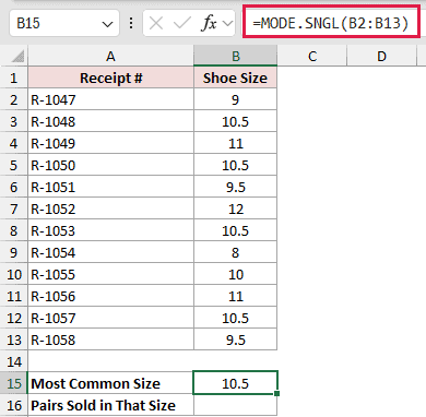
Here is the formula in B15:
=MODE.SNGL(B2:B13)
Now use B16 to count how many times the result in B15 appears in the size list:
=COUNTIF(B2:B13,B15)
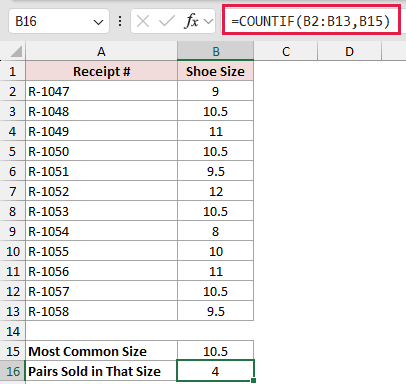
MODE.SNGL returns 10.5 because that size appears more often than any other size.
COUNTIF returns 4, confirming that four pairs were sold in size 10.5.
Example 2: Find the Mode by Category
Now let’s calculate a separate mode for each product.
Below is the dataset. Column A contains product names, while column B contains their ratings. Columns D and E list three products beside empty cells for their most common ratings.
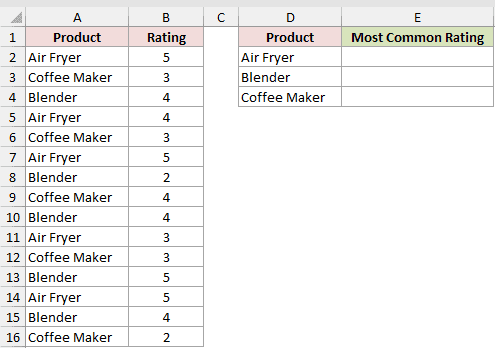
We want column E to return the most common rating for each product in column D.
Here is the formula entered in E2 and copied through E4:
=MODE.SNGL(FILTER($B$2:$B$16,$A$2:$A$16=D2))
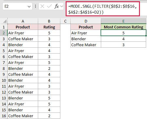
FILTER returns only the ratings for the product named in column D. MODE.SNGL then reduces those ratings to one result.
The results are 5 for Air Fryer, 4 for Blender, and 3 for Coffee Maker.
This formula needs Excel 2021, Excel 2024, or Microsoft 365 because FILTER returns a dynamic array.
Example 3: Handle Ties With MODE.MULT
Here’s where the order of your data matters.
Below is the dataset. It lists players and cleat sizes, with empty result cells for the single mode and all tied modes.
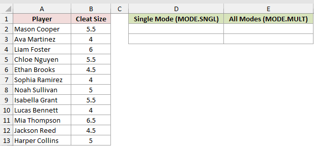
We want to see the single value MODE.SNGL selects and every value tied for the highest frequency.
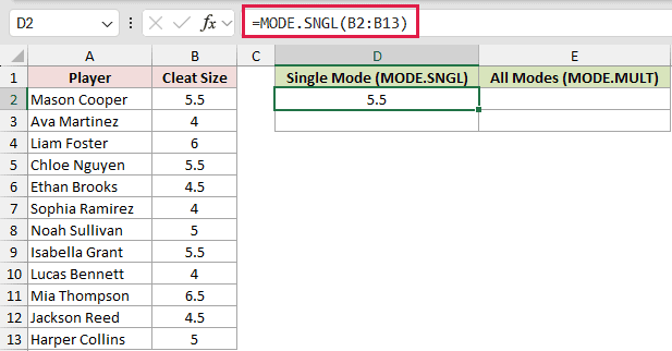
Here is the MODE.SNGL formula in D2:
=MODE.SNGL(B2:B13)
To return every tied mode, enter this formula in E2:
=MODE.MULT(B2:B13)
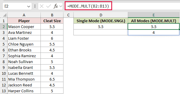
The sizes 5.5 and 4 each appear three times. MODE.SNGL returns 5.5 because it appears first, even though 4 is smaller.
MODE.MULT spills 5.5 and 4 downward in first-appearance order. Changing the row order can therefore change which tied value MODE.SNGL returns.
In Excel 2021, Excel 2024, and Microsoft 365, MODE.MULT spills automatically. Excel 2019 and earlier require a legacy array formula for multiple results.
Example 4: Handle Rows With No Repeated Score
Let’s apply MODE.SNGL across several judging rows.
Below is the dataset. Each chili has five judge scores, followed by two empty result columns for the raw mode and an error-handled result.
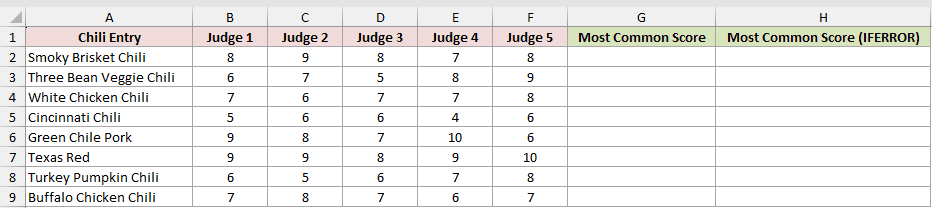
We want to find each chili’s most common score and show a friendly label when no score repeats.
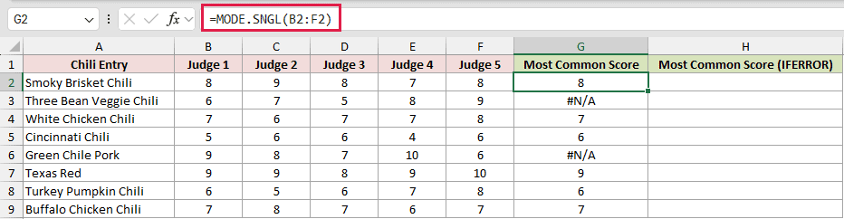
Here is the formula entered in G2 and copied through G9:
=MODE.SNGL(B2:F2)
Use IFERROR in H2 and copy it through H9 to replace the expected errors:
=IFERROR(MODE.SNGL(B2:F2),"No repeat")
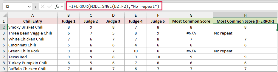
The first formula returns #N/A for Three Bean Veggie Chili and Green Chile Pork because all five scores differ.
IFERROR replaces those two errors with No repeat. Rows containing repeated scores still return their numeric modes.
Example 5: See How Zeros Change the Mode
This example shows why blanks and zeros are not interchangeable.
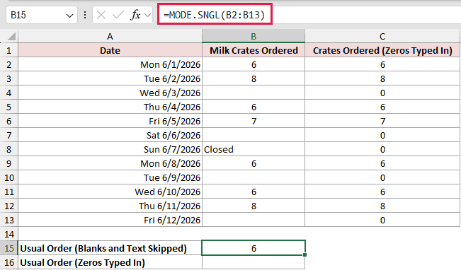
Below is the dataset. It shows daily milk-crate orders in two versions, followed by labeled empty cells for the usual order from each column.
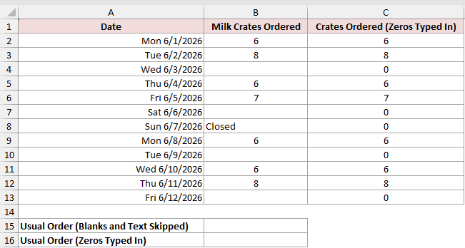
We want to compare the mode when missing entries stay blank with the mode when those entries are typed as zero.
Here is the formula for the original orders in B15:
=MODE.SNGL(B2:B13)
Here is the formula for the version containing typed zeros in B16:
=MODE.SNGL(C2:C13)
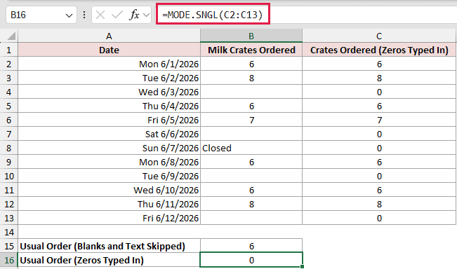
The first range contains blanks and the text Closed, which MODE.SNGL ignores. It returns 6, the most common numeric order.
Zeros are real numeric entries. In column C, zero appears five times, so it becomes the mode instead.
Pro Tip: Leave missing measurements blank unless zero is a real value. Typed zeros participate in the mode and can change the answer.
Example 6: Find the Most Common Text Value
MODE.SNGL needs a small workaround when the repeated values are text.
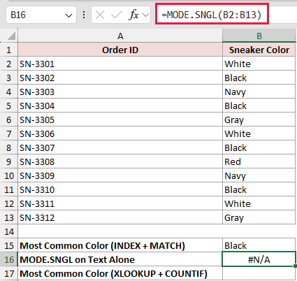
Below is the dataset. It lists sneaker orders and colors, followed by three labeled empty result cells for the INDEX approach, MODE.SNGL alone, and XLOOKUP.
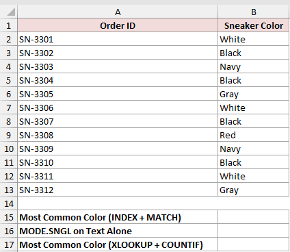
We want to return the color that appears most often and compare two working approaches with MODE.SNGL alone.
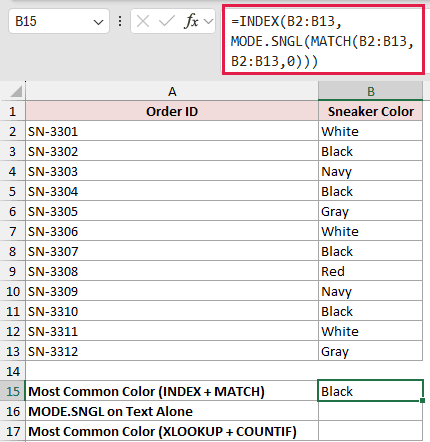
Here is the INDEX and MATCH formula in B15:
=INDEX(B2:B13,MODE.SNGL(MATCH(B2:B13,B2:B13,0)))
In Excel 2019 and earlier, confirm the B15 formula with Ctrl+Shift+Enter. In Excel 2021, Excel 2024, and Microsoft 365, press Enter.
For comparison, enter MODE.SNGL directly on the text range in B16:
=MODE.SNGL(B2:B13)
The newer XLOOKUP approach in B17 is another option:
=XLOOKUP(MAX(COUNTIF(B2:B13,B2:B13)),COUNTIF(B2:B13,B2:B13),B2:B13)
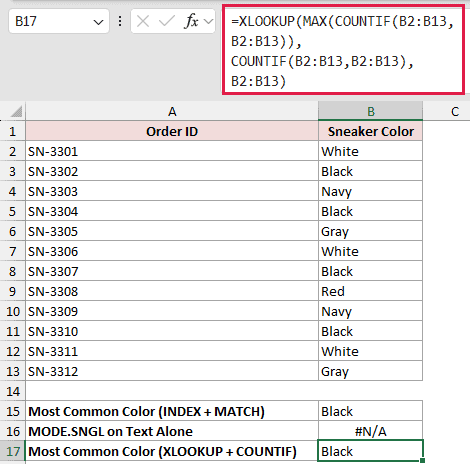
MATCH converts each color to its first position. MODE.SNGL finds the most frequent position, and INDEX returns Black from that position.
MODE.SNGL alone returns #N/A because the range contains only text.
The XLOOKUP version also returns Black. It finds the largest COUNTIF result, then returns the first color with that count.
The XLOOKUP approach is available in Excel 2021, Excel 2024, and Microsoft 365.
Example 7: Compare Mode, Median, and Average
Let’s finish with a list containing two unusually large orders.
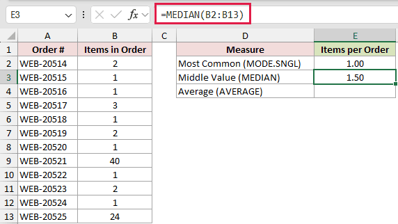
Below is the dataset. It lists order numbers and item counts, with three labeled empty cells for the mode, median, and average.
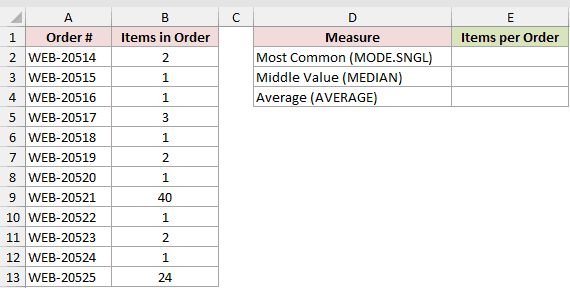
We want to compare three summaries and decide which one best describes a typical order.
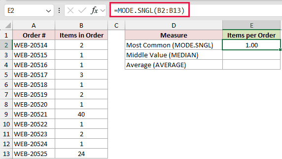
Here is the MODE.SNGL formula in E2:
=MODE.SNGL(B2:B13)
Here is the MEDIAN formula in E3:
=MEDIAN(B2:B13)
Here is the AVERAGE formula in E4:
=AVERAGE(B2:B13)
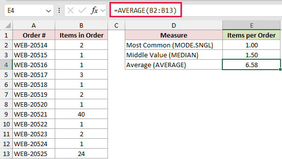
MODE.SNGL returns 1.00 because 1 occurs six times in the 12 orders.
MEDIAN returns 1.50, the average of the two middle sorted values, 1 and 2.
AVERAGE returns 6.58 because the bulk orders of 40 and 24 pull it upward.
Here, the mode best describes a typical order because six of the 12 orders are one item. The 40-item and 24-item orders pull the average to 6.58.
Tips & Common Mistakes
- MODE.SNGL returns #N/A when no numeric value repeats. Wrap it with IFERROR when a descriptive label would be clearer.
- When frequencies tie, MODE.SNGL returns the tied value that appears first, not necessarily the smallest value.
- Text, blank cells, and logical values inside a range are ignored. Numeric zeros are included.
- MODE.SNGL reduces a range or array to one result. It can evaluate an array returned by FILTER, but it does not spill by itself.
- Use MODE.MULT when you need every tied mode instead of a single result.
- MODE is the older compatibility function and returns the same result as MODE.SNGL.
This article covered how MODE.SNGL handles ties, zeros, grouped data, and rows without repeats.
It also showed how to return a common text value and compare mode with median and average.
Related Excel Functions / Articles:
