FORECAST.ETS.CONFINT Function in Excel

Excel’s FORECAST.ETS.CONFINT function returns a confidence radius around an ETS point forecast for a specified future date.

The radius is the distance from the forecast, not either boundary. Subtract the radius for the lower bound and add it for the upper bound.

The seasonality, data completion, and aggregation settings should match those used by FORECAST.ETS. Otherwise, the radius and point forecast describe different models.

I’ll build a six-month forecast band, compare confidence levels, test seasonality settings, and show how missing observations affect the result.

FORECAST.ETS.CONFINT Function Syntax in Excel

The syntax of the FORECAST.ETS.CONFINT function is:

=FORECAST.ETS.CONFINT(target_date, values, timeline, [confidence_level], [seasonality], [data_completion], [aggregation])

• target_date is the future date or numeric point for which you want the radius.
• values contains the historical values used by the forecast model.
• timeline contains the matching dates or numeric points at a consistent, nonzero interval.
• [confidence_level] is a number greater than 0 and less than 1. The default is 0.95.
• [seasonality] is 1 for automatic detection, 0 for no seasonality, or a positive whole number for a fixed cycle length.
• [data_completion] is 1 by default to complete missing points with neighboring averages. Use 0 to treat them as zero.
• [aggregation] is 1 for AVERAGE, 2 for COUNT, 3 for COUNTA, 4 for MAX, 5 for MEDIAN, 6 for MIN, or 7 for SUM.

When to Use FORECAST.ETS.CONFINT Function

• Add lower and upper confidence bounds to an ETS forecast.
• Compare how different confidence levels change the forecast radius.
• Measure uncertainty around seasonal forecasts for sales, orders, tickets, or revenue.
• Compare automatic, fixed, and no-seasonality model settings.
• Test how Excel’s missing-data setting changes the forecast band.

Example 1: Build a Six-Month Forecast Band

We’ll start with the complete forecast-band workflow.

Below is the dataset with 36 months of store orders and an empty six-month output table for January through June 2026.

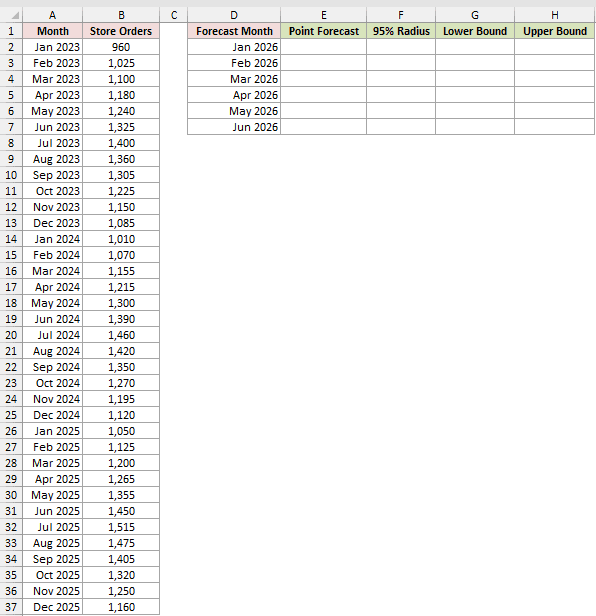
I want the point forecast, 95% radius, lower bound, and upper bound for each future month.

Here is the point-forecast formula entered in E2, spilling through E7:

=FORECAST.ETS(D2:D7,$B$2:$B$37,$A$2:$A$37,12,1,1)

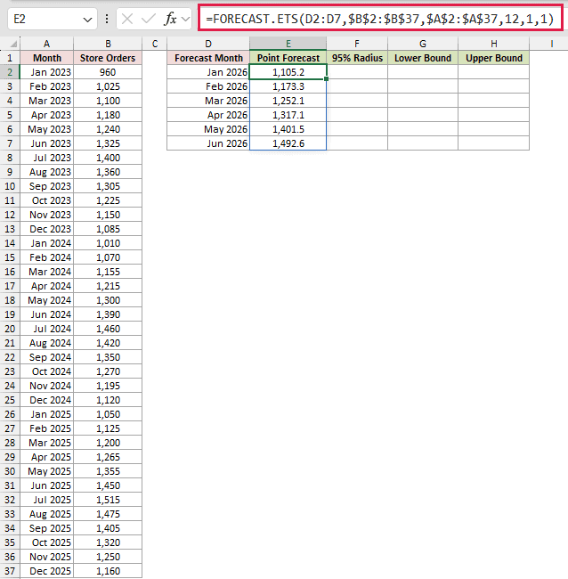
The FORECAST.ETS function uses a 12-month seasonal cycle. Its six point forecasts spill into E2:E7.

Now I need a matching radius for each target month.

Here is the radius formula entered in F2, spilling through F7:

=MAP(D2:D7,LAMBDA(target_month,FORECAST.ETS.CONFINT(target_month,$B$2:$B$37,$A$2:$A$37,0.95,12,1,1)))

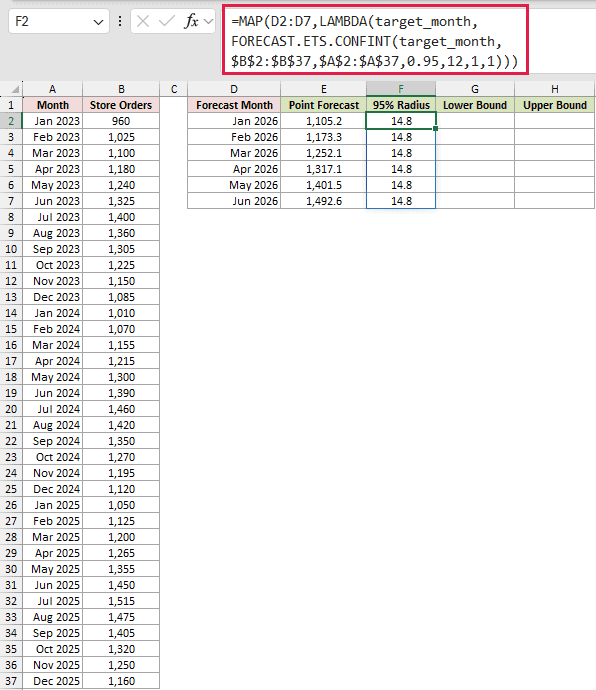
MAP calls FORECAST.ETS.CONFINT once for each date in D2:D7. Every returned radius is 14.8 in this dataset.

Next, I can subtract the radius from each point forecast.

Here is the lower-bound formula entered in G2 and filled down to G7:

=E2-F2

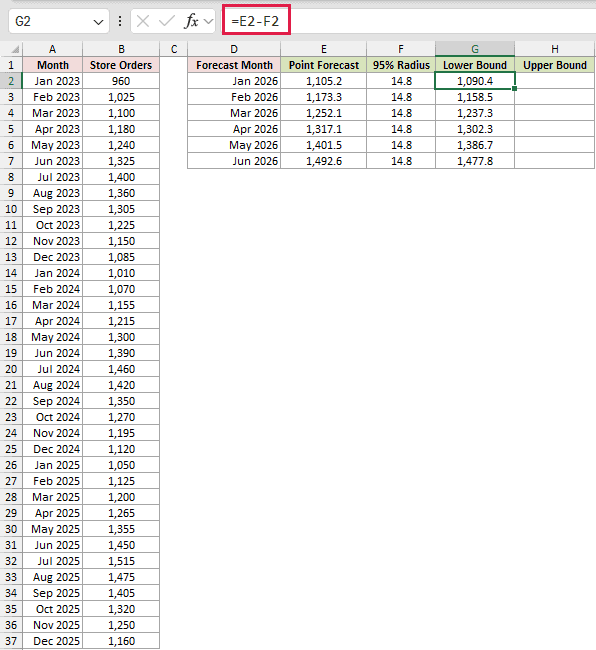
The lower bound for January 2026 is 1,090.4, calculated from the 1,105.2 forecast minus the 14.8 radius.

Finally, I can add the radius to each point forecast.

Here is the upper-bound formula entered in H2 and filled down to H7:

=E2+F2

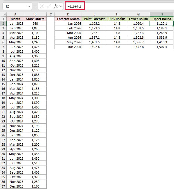
The upper bound for January is 1,120.1. Together, columns G and H form the confidence band around the forecasts in column E.

Excel uses the stored, unrounded values. With one-decimal display, a shown bound can differ by 0.1 from arithmetic using the displayed forecast and radius.

Pro Tip: MAP is available in Microsoft 365 and Excel 2024. In other supported desktop versions, calculate one target date per row and fill the scalar formulas down.

Example 2: Compare 80% to 99% Confidence

The confidence level controls how wide the radius becomes.

Below is the ticket history in A:B, forecast settings in D:E, and an empty confidence comparison table in G:J.

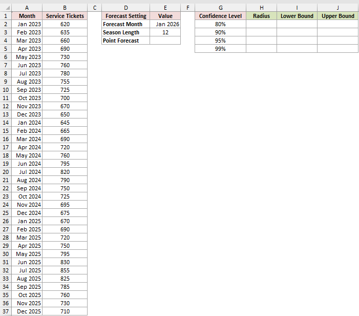
I want one January 2026 forecast and four bands using 80%, 90%, 95%, and 99% confidence levels.

Here is the point-forecast formula entered in E4:

=FORECAST.ETS(E2,$B$2:$B$37,$A$2:$A$37,E3,1,1)

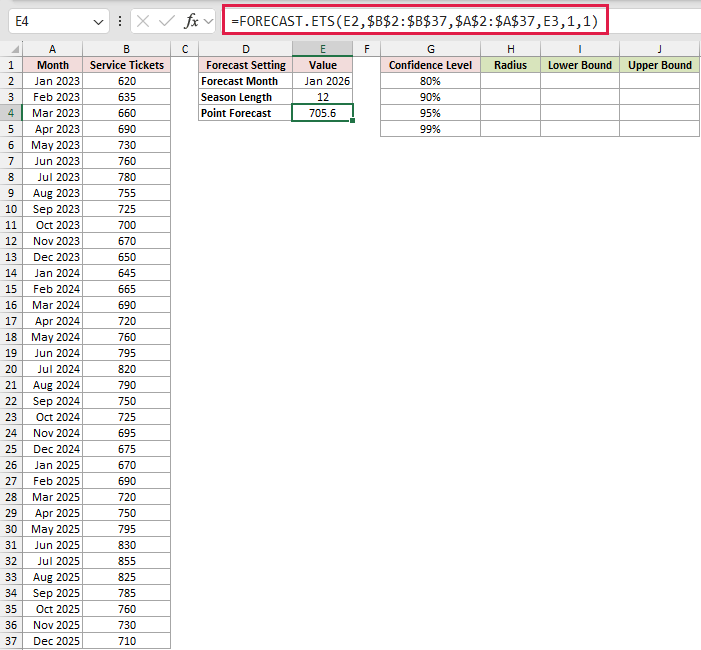
The formula returns 705.6. Every confidence row uses this same point forecast and the same season length of 12.

Here is the radius formula entered in H2 and filled down to H5:

=FORECAST.ETS.CONFINT($E$2,$B$2:$B$37,$A$2:$A$37,G2,$E$3,1,1)

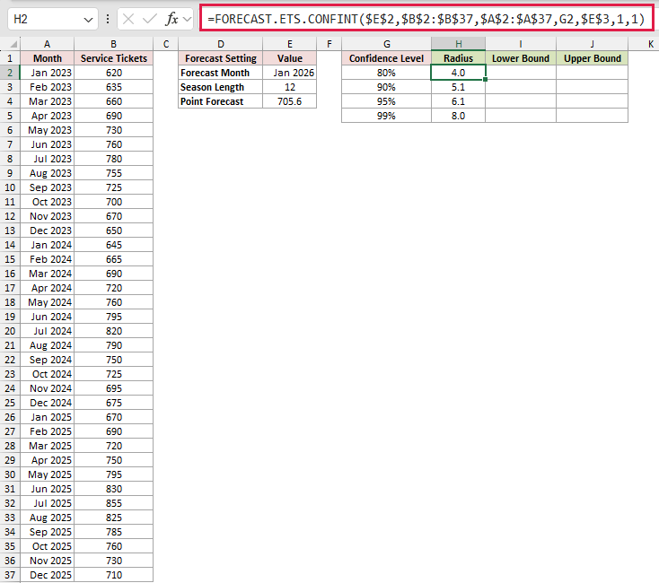
The radius increases from 4.0 at 80% to 5.1, 6.1, and 8.0 as the confidence level rises.

Here is the lower-bound formula entered in I2 and filled down to I5:

=$E$4-H2

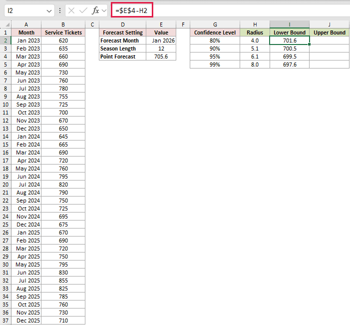
The lower bounds decrease from 701.6 at 80% to 697.6 at 99% because each larger radius extends farther below the forecast.

Here is the upper-bound formula entered in J2 and filled down to J5:

=$E$4+H2

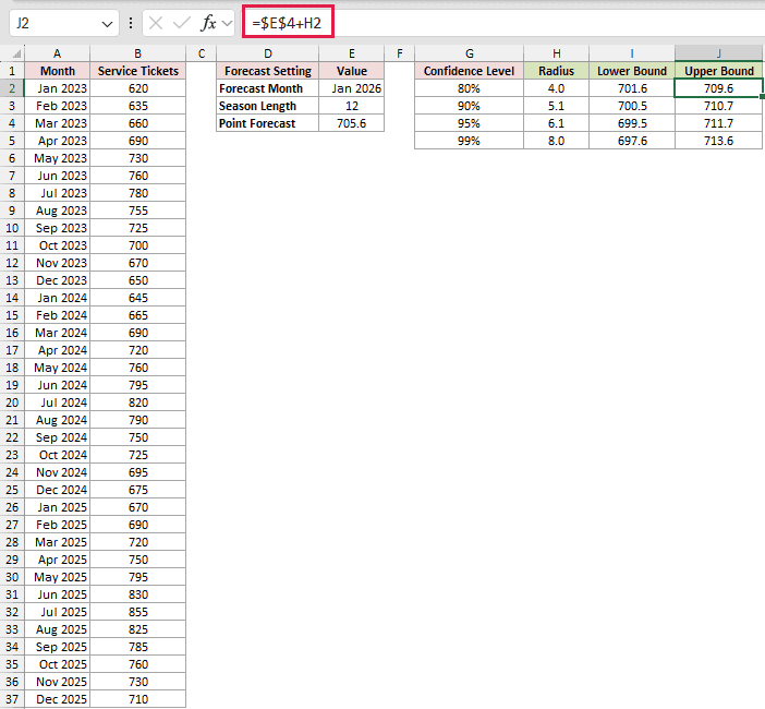
The upper bounds rise from 709.6 to 713.6. A higher confidence level produces a wider band around the same forecast.

Example 3: Compare Seasonality Settings

FORECAST.ETS and FORECAST.ETS.CONFINT must use the same seasonality choice.

Below is 36 months of subscription revenue. The forecast date is in E1, while the output headers begin in row 2.

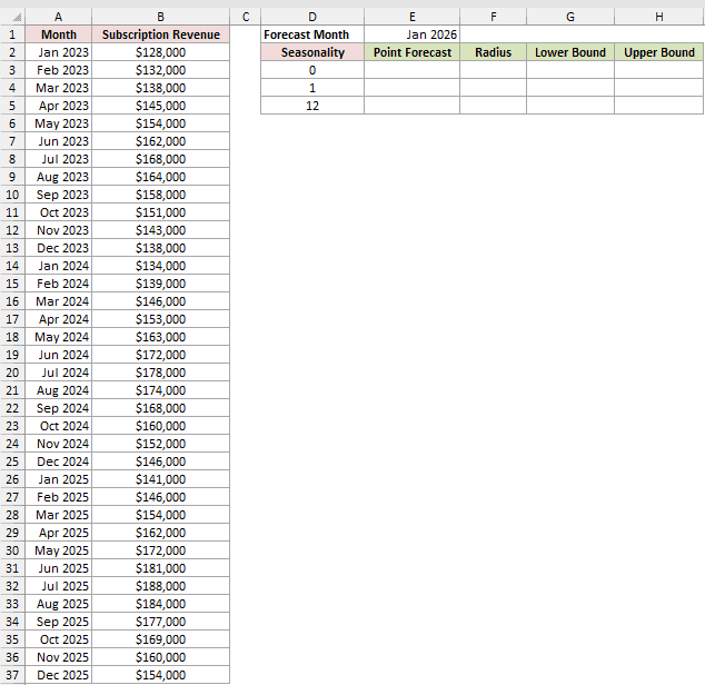
I want to compare no seasonality, automatic detection, and a fixed 12-month cycle for January 2026.

Here is the point-forecast formula entered in E3 and filled down to E5:

=FORECAST.ETS($E$1,$B$2:$B$37,$A$2:$A$37,D3,1,1)

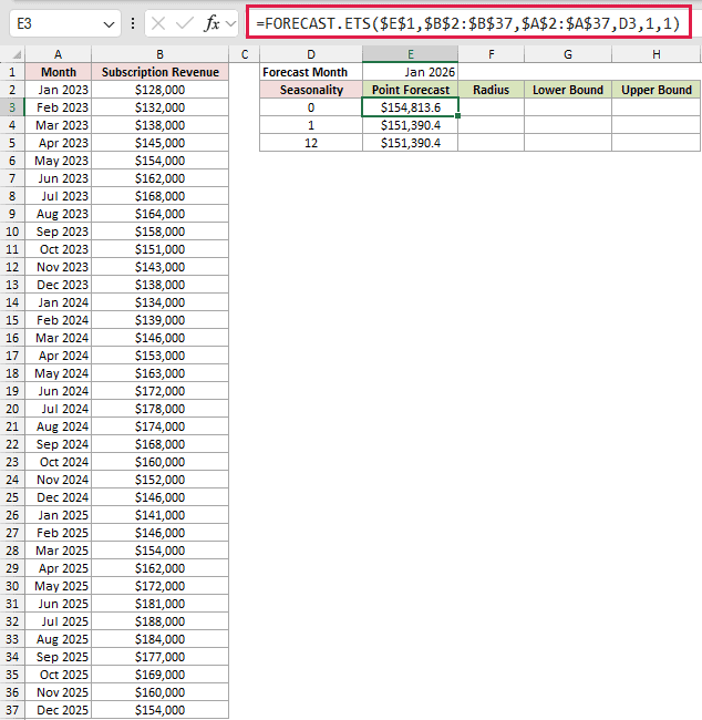
Column D supplies the seasonality setting. 0 removes seasonality, 1 asks Excel to detect it, and 12 sets a 12-month cycle.

Here is the radius formula entered in F3 and filled down to F5:

=FORECAST.ETS.CONFINT($E$1,$B$2:$B$37,$A$2:$A$37,0.95,D3,1,1)

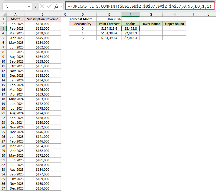
The no-seasonality model returns a forecast of $154,813.6 with an $8,475.8 radius.

Automatic and fixed-12 seasonality both return $151,390.4 with a $2,013.3 radius for this series.

Here is the lower-bound formula entered in G3 and filled down to G5:

=E3-F3

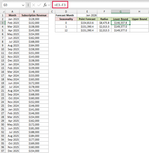
The lower bounds are $146,337.8 for seasonality 0 and $149,377.0 for settings 1 and 12.

Here is the upper-bound formula entered in H3 and filled down to H5:

=E3+F3

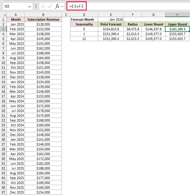
The corresponding upper bounds are $163,289.5 and $153,403.7.

The 36-month history gives the model three annual cycles to work with. That is a deliberate sample design here, not an official Excel minimum.

Example 4: Compare Missing-Data Settings

This example shows what data_completion changes inside the ETS model.

The history contains 35 observations and skips the July 2024 timestamp. The January 2026 target date sits separately in J2.

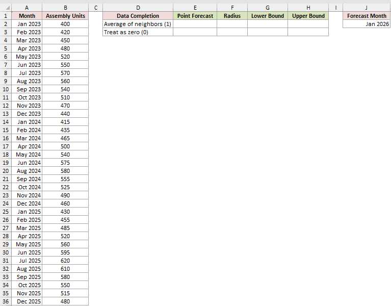
I want to compare interpolation, which averages the neighboring observations, with treating the missing observation as zero.

Here is the point-forecast formula entered in E2 and filled down to E3:

=FORECAST.ETS($J$2,$B$2:$B$36,$A$2:$A$36,12,IF(D2="Average of neighbors (1)",1,0),1)

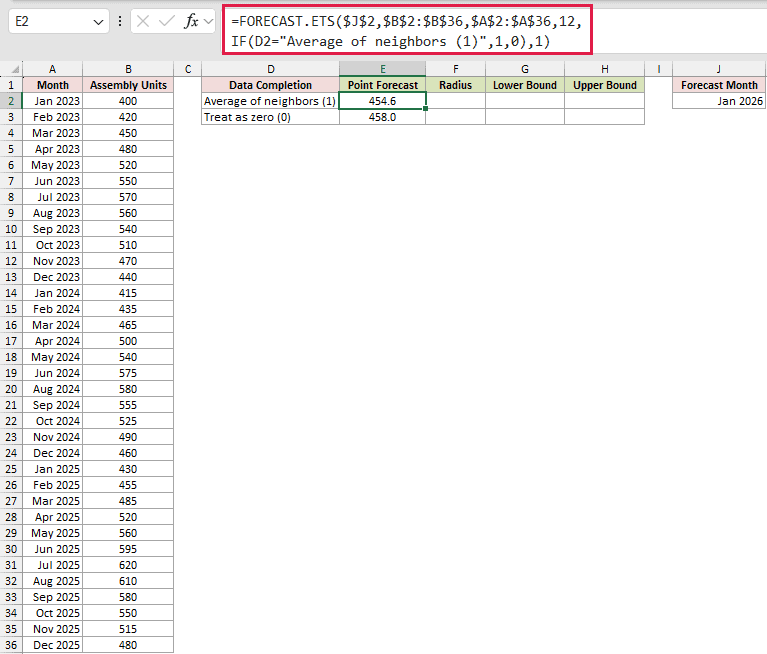
The IF function converts each label in column D to the matching data-completion setting.

Neighbor averaging returns a point forecast of 454.6. Treating the missing point as zero returns 458.0.

Here is the radius formula entered in F2 and filled down to F3:

=FORECAST.ETS.CONFINT($J$2,$B$2:$B$36,$A$2:$A$36,0.95,12,IF(D2="Average of neighbors (1)",1,0),1)

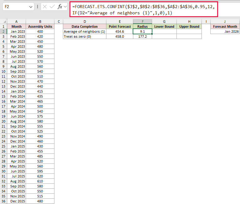
The radius is 9.1 with neighbor averaging and 177.2 when the missing point is treated as zero.

This difference comes from the model’s data-completion choice. The formula does not insert a visible July row into the source timeline.

Here is the lower-bound formula entered in G2 and filled down to G3:

=E2-F2

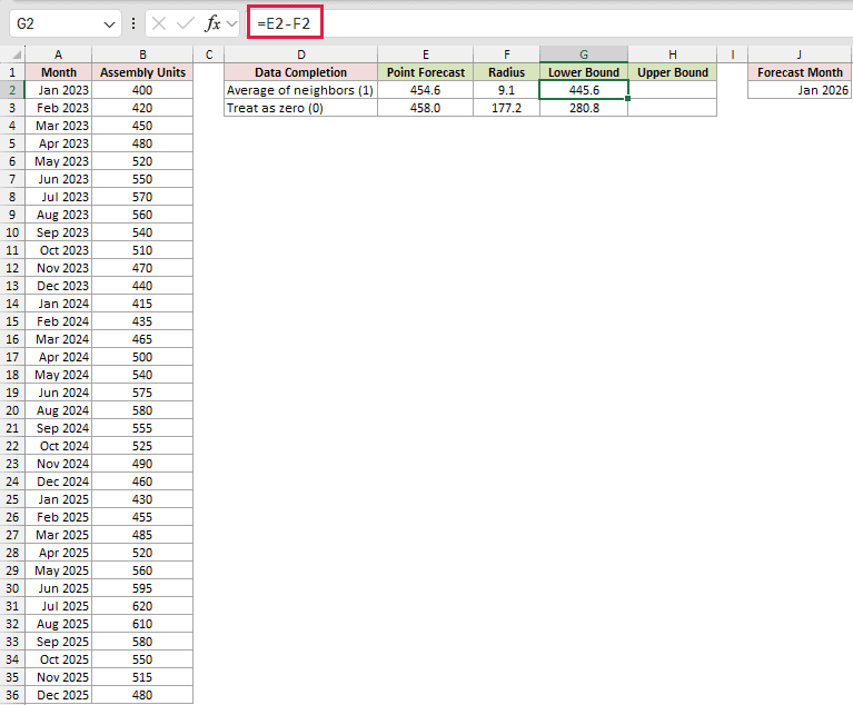
The lower bound is 445.6 with neighbor averaging and 280.8 when Excel treats the missing point as zero.

Here is the upper-bound formula entered in H2 and filled down to H3:

=E2+F2

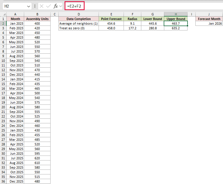
The upper bounds are 463.7 and 635.2, respectively.

Pro Tip: Microsoft documents support for up to 30% missing data. Use the same data-completion setting in FORECAST.ETS and FORECAST.ETS.CONFINT.

Tips & Common Mistakes

• Treat the function’s result as a radius. Calculate the lower bound as forecast-radius and the upper bound as forecast+radius.
• Keep the seasonality, data completion, and aggregation arguments identical in FORECAST.ETS and FORECAST.ETS.CONFINT.
• Use a target date after the final historical date. An earlier target returns #NUM!.
• Keep values and timeline the same size. Mismatched ranges return #N/A.
• Use timeline dates or numbers with a consistent, nonzero interval. Excel sorts the timeline internally before calculating.
• Enter a confidence level strictly between 0 and 1. Values outside that range return #NUM!.
• The maximum supported seasonality is 8,760. A larger value returns #NUM!.
• FORECAST.ETS.CONFINT works in supported desktop Excel releases. Microsoft says it is unavailable in Excel for the web, iOS, and Android.

I covered forecast-band arithmetic, confidence sensitivity, seasonality choices, and missing-data handling with FORECAST.ETS.CONFINT.

I hope you found this article helpful.

List of All Excel Functions

Related Excel Functions / Articles:

• FORECAST.ETS.SEASONALITY Function in Excel
• FORECAST.LINEAR Function in Excel
• FORECAST Function in Excel
• FORECAST.ETS.STAT function