FORECAST.ETS.STAT Function in Excel

The FORECAST.ETS.STAT function in Excel returns statistics about an exponential smoothing forecast model, including its historical errors, smoothing parameters, and timeline step size.

A forecast can look reasonable without fitting your history well. These statistics help you check that fit and see how seasonality or missing-data settings change it.

FORECAST.ETS calculates the future estimate. FORECAST.ETS.STAT examines the model built from the same history and settings, so you can judge the estimate with more context.

I’ll show you how to interpret the statistics, compare seasonal settings, and spot a missing-data choice that makes the model fit worse.

FORECAST.ETS.STAT Function Syntax in Excel

The function uses historical values, their timeline, and a code identifying the statistic you want.

=FORECAST.ETS.STAT(values, timeline, statistic_type, [seasonality], [data_completion], [aggregation])

• values (required): The historical numbers you want to model.
• timeline (required): The corresponding numeric dates or periods. The ranges must have matching sizes, and Excel must be able to identify a consistent step.
• statistic_type (required): The statistic code from the table below.
• seasonality (optional): Use 1, the default, for automatic detection; 0 for no seasonality; or a cycle length such as 12 for a yearly pattern in monthly data.
• data_completion (optional): Use 1, the default, to estimate missing points from neighboring values. Use 0 to treat missing points as zero.
• aggregation (optional): Controls how Excel combines values sharing a timestamp. Omitted or 1 means AVERAGE. An explicit 0 returns #NUM!.

Statistic type	Returned statistic	What it describes
1	Alpha	Level smoothing parameter
2	Beta	Trend smoothing parameter
3	Gamma	Seasonal smoothing parameter
4	MASE	Mean absolute scaled error
5	SMAPE	Symmetric mean absolute percentage error
6	MAE	Mean absolute error
7	RMSE	Root mean squared error
8	Step size	Detected spacing in the timeline

Type 8 is the step size, not a confidence value. For a forecast confidence interval, the related function is FORECAST.ETS.CONFINT.

When to Use FORECAST.ETS.STAT Function

• Check how well an ETS model fits historical signups, orders, or usage before relying on its forecast.
• Compare automatic seasonality with a cycle length you already know.
• Compare forecast errors across series with very different volumes.
• Check timeline spacing or investigate a missing-data setting.

Example 1: Return All Forecast Statistics Together

Let’s start with a statistics panel beside weekly web orders.

Below is the dataset. Columns A:B hold weekly dates and orders; D:E list statistic codes and names, with column F reserved for their values.

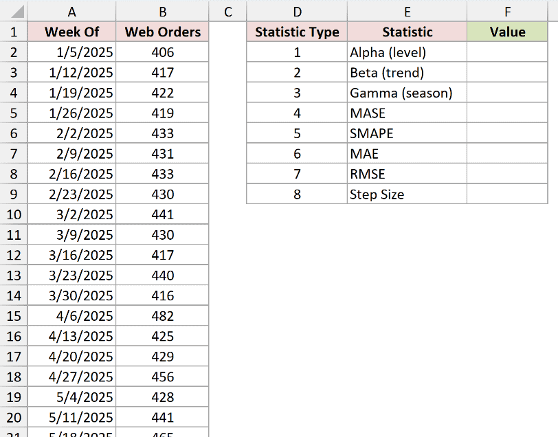
We want to calculate every listed statistic from the same order history.

Enter this formula in F2:

=FORECAST.ETS.STAT($B$2:$B$53,$A$2:$A$53,D2:D9)

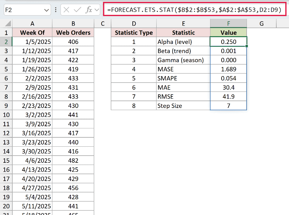
Each statistic summarizes the entire history. Passing the code range D2:D9 returns a separate statistic for each code, spilling into F2:F9.

This spill works in desktop Excel 2021, Excel 2024, and Microsoft 365. In Excel 2019 and earlier supported versions, use individual statistic-cell references and fill down.

Statistic	Displayed result
Alpha	0.250
Beta	0.001
Gamma	0.000
MASE	1.689
SMAPE	0.054
MAE	30.4
RMSE	41.9
Step Size	7

Alpha, beta, and gamma describe smoothing of the level, trend, and seasonal pattern. They aren’t accuracy scores, so don’t rank the model by those values.

MASE below 1 means the model beats the naive forecast on the historical data. Here, 1.689 fails that check, even though the formula calculates normally.

MAE of 30.4 and RMSE of 41.9 are measured in orders. RMSE gives larger misses more weight, while MAE describes the average absolute miss.

SMAPE is the fraction 0.054. You can format that cell as a percentage; the function itself returns a fraction.

The step size is 7, because the dates advance weekly and Excel measures date spacing in days.

Pro Tip: Microsoft’s Forecast Sheet can include the same model statistics as static values when you select Include forecast statistics. Use formulas when you want the statistics to recalculate with the inputs.

Example 2: Check Fit Beside a Signup Forecast

Now let’s put the fit check beside the estimate you’ll actually use.

Below is the dataset. A:B contain monthly new signups. The D:E panel has a typed Next Month input in E2 and labeled spaces for forecast diagnostics.

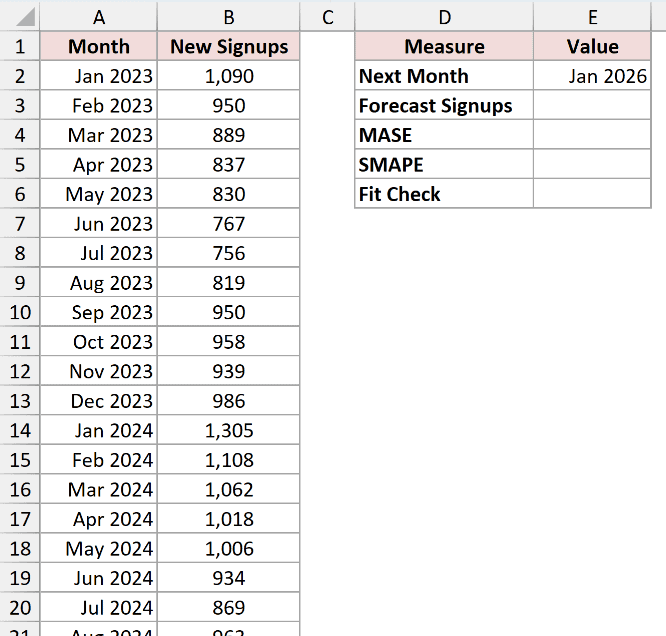
We want to forecast the next month’s signups and check the historical fit of that same seasonal model.

Enter the forecast formula in E3:

=FORECAST.ETS(E2,$B$2:$B$37,$A$2:$A$37,12)

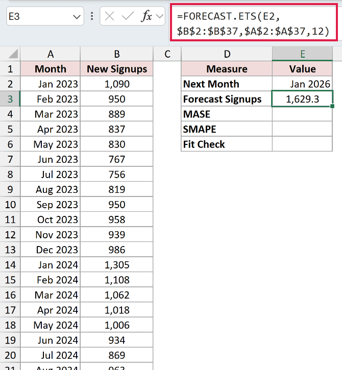
For the Jan 2026 input, the forecast displays 1,629.3 signups. The seasonality argument uses a 12-month cycle.

Calculate MASE in E4:

=FORECAST.ETS.STAT($B$2:$B$37,$A$2:$A$37,4,12)

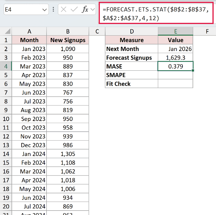
The result is 0.379, below 1. This model beats the naive forecast on the historical data.

Next, calculate SMAPE in E5:

=FORECAST.ETS.STAT($B$2:$B$37,$A$2:$A$37,5,12)

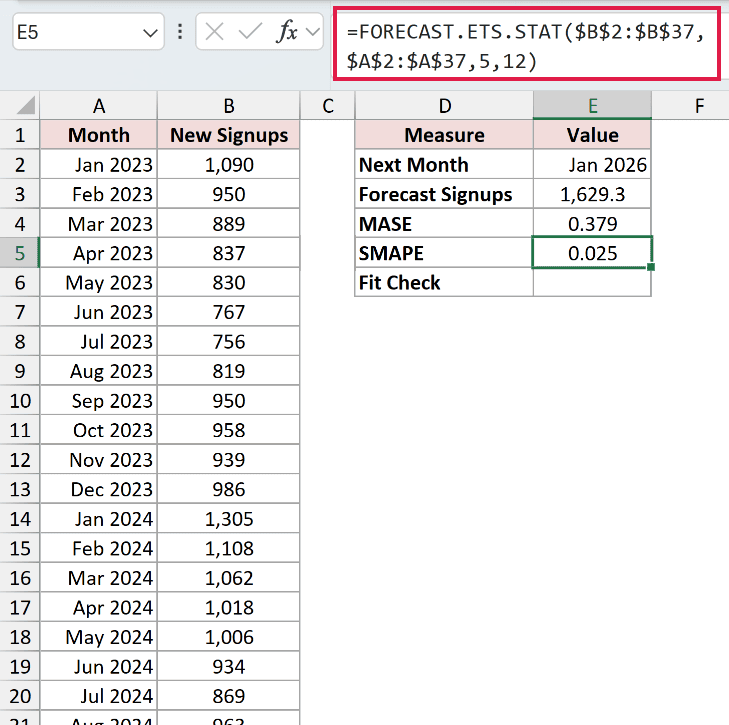
SMAPE displays 0.025, a relative error expressed as a fraction. Both diagnostic formulas use the same history and seasonality as the forecast.

Finally, turn the MASE check into a readable label in E6:

=IF(E4<1,"Beats naive forecast","Weak fit")

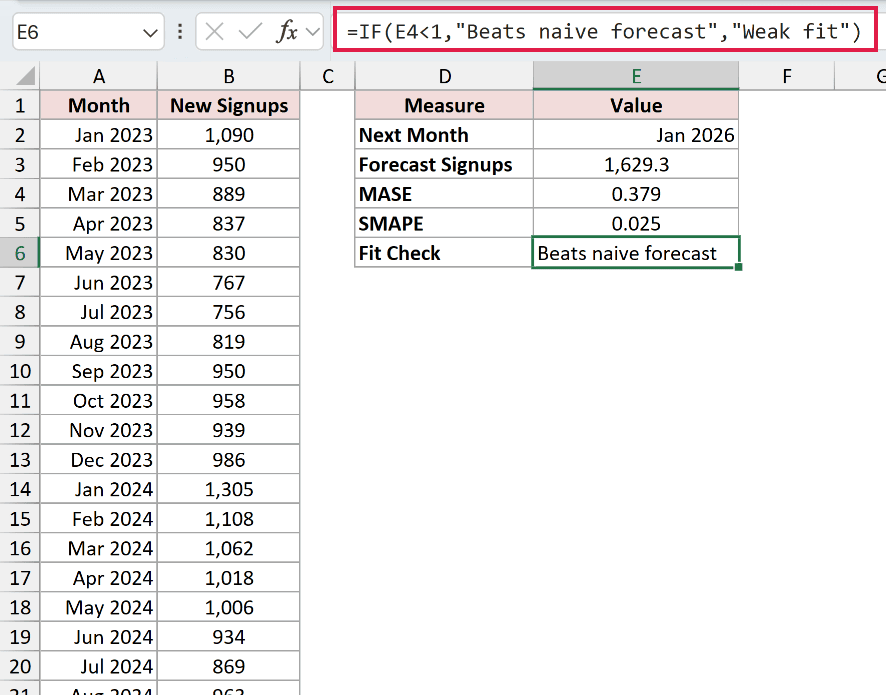
E6 returns Beats naive forecast. IF reads the calculated MASE in E4, so the label updates when the history changes.

Pro Tip: This label describes historical fit, not guaranteed future accuracy. Keep the history, seasonality, data completion, and aggregation settings consistent between FORECAST.ETS and FORECAST.ETS.STAT.

Example 3: Compare Seasonality Settings by Error

A seasonal pattern can be easier to judge when you compare its errors directly.

Below is the dataset. A:B contain monthly household electricity usage. D lists seasonality settings, and E:G provide labeled columns for MASE, SMAPE, and RMSE.

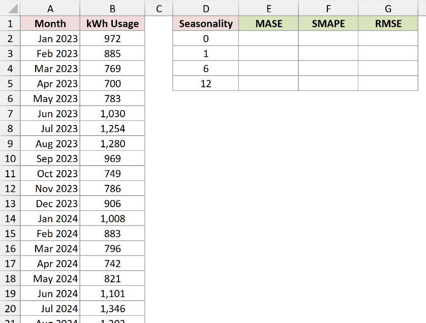
We want to compare each seasonality setting against the same usage history.

Enter the MASE formula in E2 and copy it down through E5:

=FORECAST.ETS.STAT($B$2:$B$37,$A$2:$A$37,4,D2)

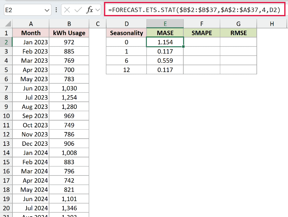
The locked history ranges stay fixed, while D2 changes as you copy down.

Enter SMAPE in F2 and copy it down through F5:

=FORECAST.ETS.STAT($B$2:$B$37,$A$2:$A$37,5,D2)

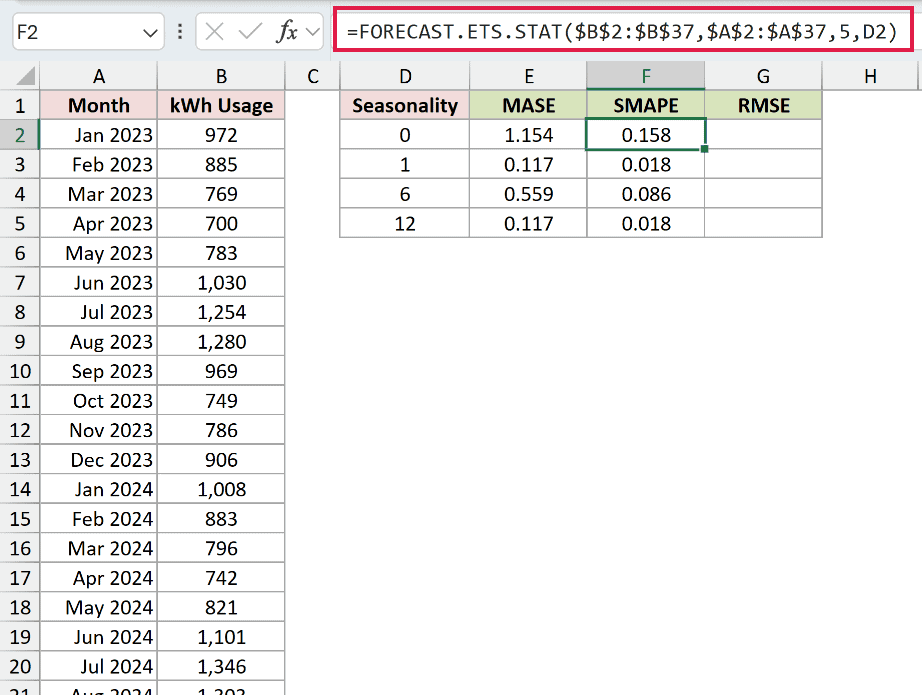
Then enter RMSE in G2 and copy it down through G5:

=FORECAST.ETS.STAT($B$2:$B$37,$A$2:$A$37,7,D2)

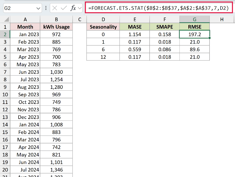
Here’s the completed comparison. Lower errors indicate a better fit to this history.

Seasonality	MASE	SMAPE	RMSE
0	1.154	0.158	197.2
1	0.117	0.018	21.0
6	0.559	0.086	89.6
12	0.117	0.018	21.0

Turning seasonality off produces the largest errors. The 6-month cycle improves the fit, but the yearly cycle fits better.

The automatic setting, 1, matches the 12 row because auto-detection found a 12-month cycle. These matching results are expected.

FORECAST.ETS.SEASONALITY is the companion function for inspecting the detected cycle length. STAT lets you compare how well different choices fit.

Example 4: Check the Timeline Step Size

The same usage values can behave differently when you change their timeline.

Below is the dataset. A:D contain weekly dates, week numbers, meter-read dates, and electricity usage. F:G hold timeline labels and spaces for step-size checks.

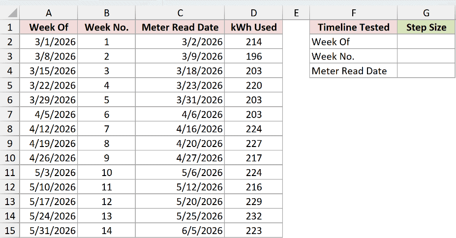
We want to check which timelines provide consistent spacing for the model.

Test the weekly dates in G2:

=FORECAST.ETS.STAT($D$2:$D$15,A2:A15,8)

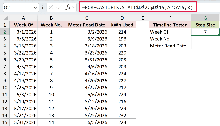
The result is 7. These dates are separated by 7 days.

Test the week-number timeline in G3:

=FORECAST.ETS.STAT($D$2:$D$15,B2:B15,8)

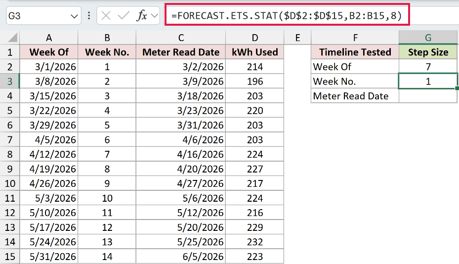
The result is 1, because the week numbers advance by 1. Step size follows the timeline’s units, not the units of electricity usage.

For the deliberate error demonstration, test the irregular meter-read dates in G4:

=FORECAST.ETS.STAT($D$2:$D$15,C2:C15,8)

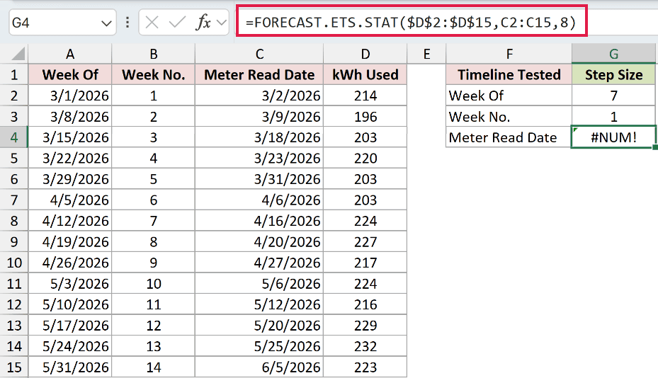
G4 deliberately returns #NUM! because Excel can’t find a constant step in this timeline.

Check whether your dates identify the periods being measured or merely when someone recorded them. Here, the regular Week Of column identifies the usage periods.

Example 5: Compare Channels of Different Sizes

A large order channel can have larger errors in orders while fitting better in relative terms.

Below is the dataset. A:C hold monthly website and wholesale orders. E:I contain channel labels and spaces for their error statistics.

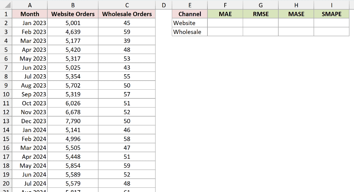
We want to compare each channel using both errors in orders and scale-free errors.

Calculate website MAE in F2:

=FORECAST.ETS.STAT($B$2:$B$37,$A$2:$A$37,6)

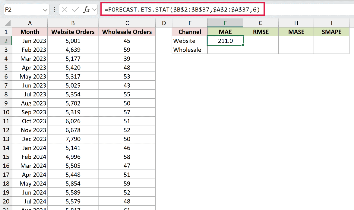
The website MAE is 211.0 orders.

Calculate website RMSE in G2:

=FORECAST.ETS.STAT($B$2:$B$37,$A$2:$A$37,7)

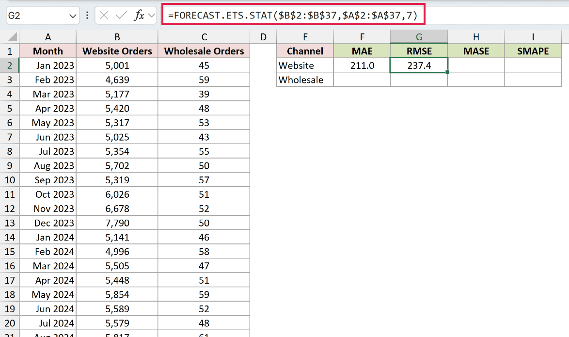
The website RMSE is 237.4 orders.

Calculate website MASE in H2:

=FORECAST.ETS.STAT($B$2:$B$37,$A$2:$A$37,4)

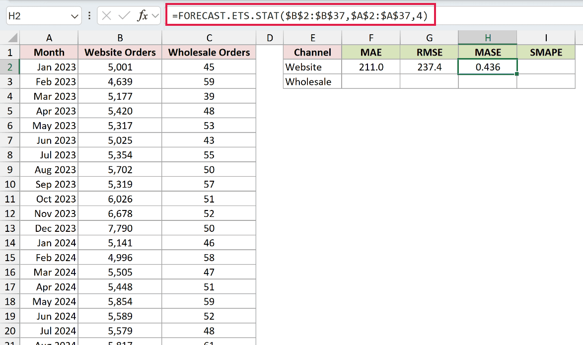
Website MASE is 0.436, below the naive benchmark.

Calculate website SMAPE in I2:

=FORECAST.ETS.STAT($B$2:$B$37,$A$2:$A$37,5)

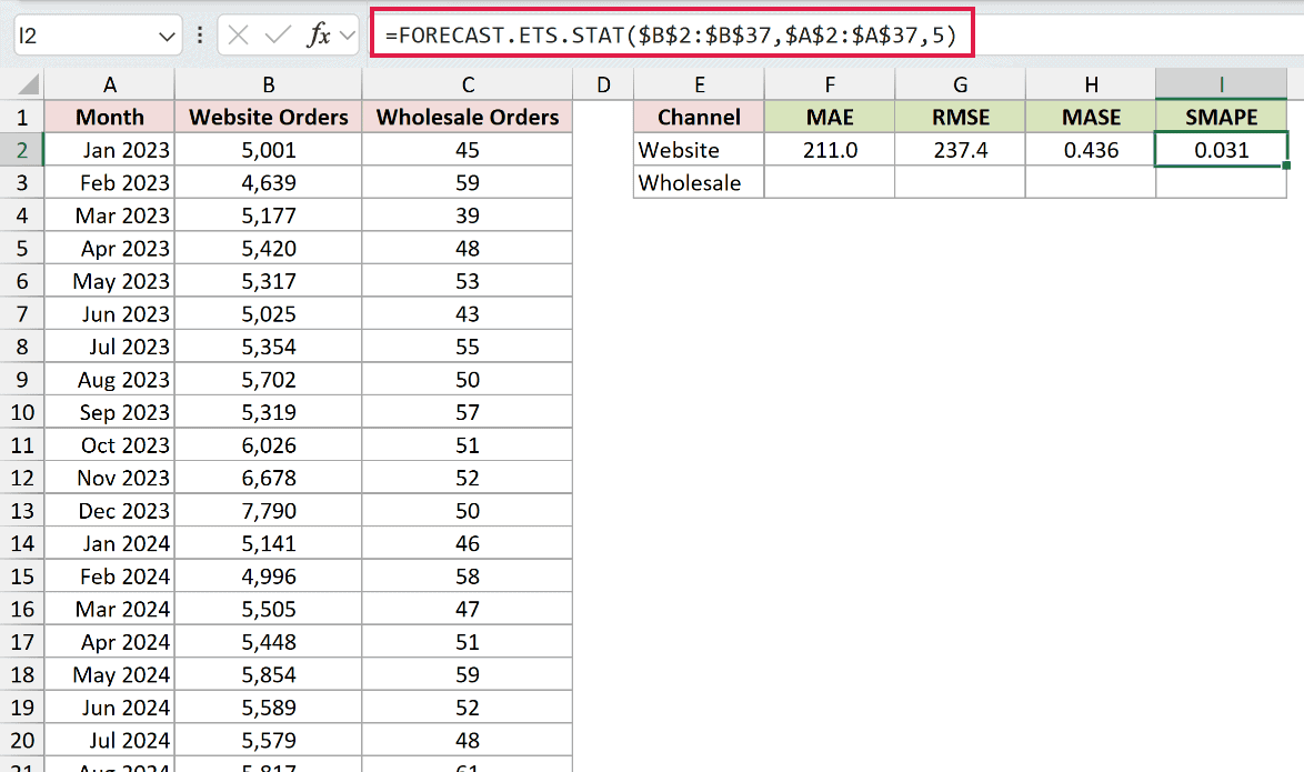
Website SMAPE is 0.031, expressed as a fraction.

For the wholesale comparison, calculate MAE in F3:

=FORECAST.ETS.STAT($C$2:$C$37,$A$2:$A$37,6)

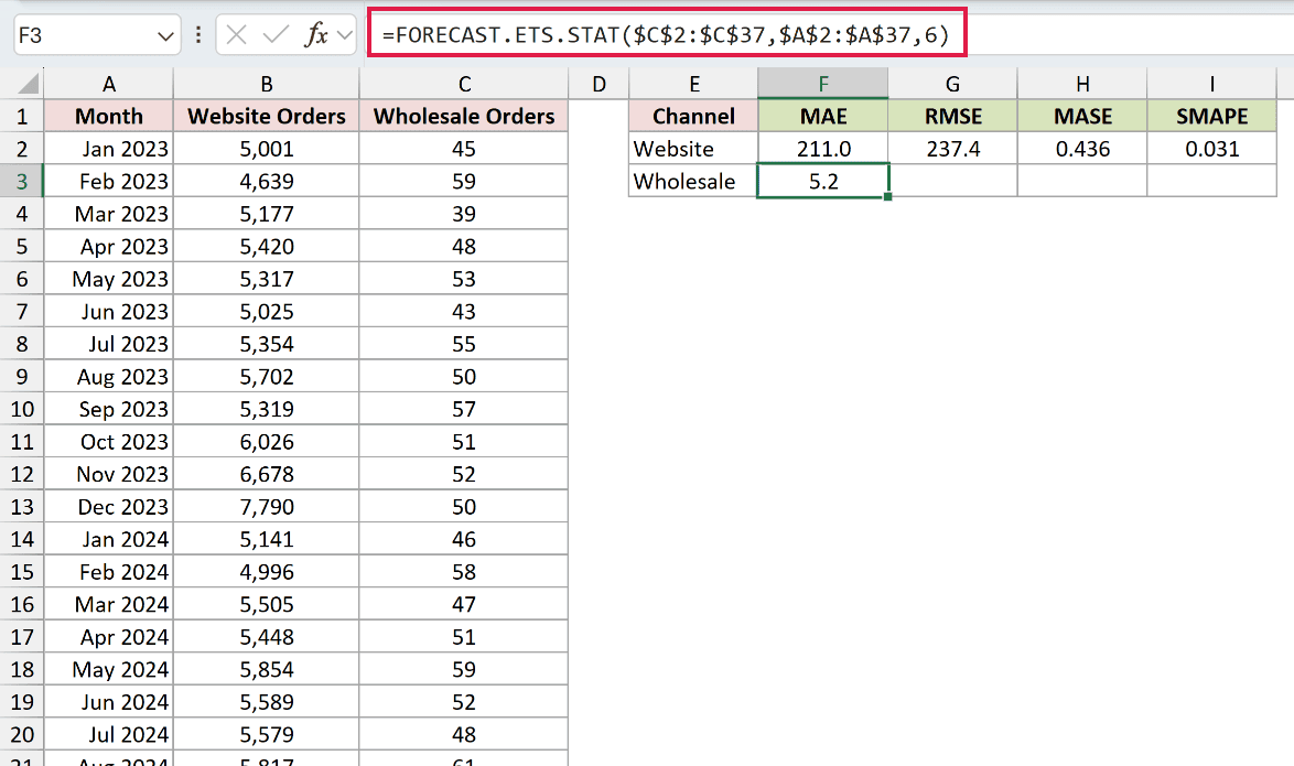
Wholesale MAE is 5.2 orders. Its smaller order volume makes this absolute error look much smaller.

Calculate wholesale RMSE in G3:

=FORECAST.ETS.STAT($C$2:$C$37,$A$2:$A$37,7)

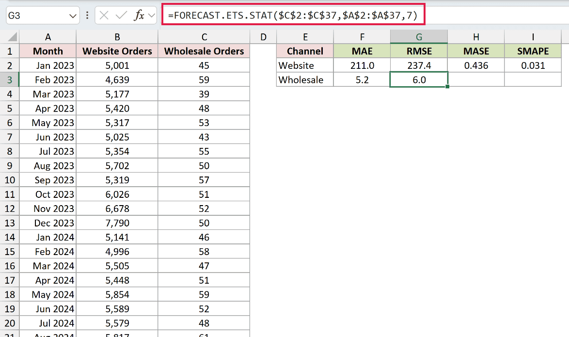
Wholesale RMSE is 6.0 orders.

Calculate wholesale MASE in H3:

=FORECAST.ETS.STAT($C$2:$C$37,$A$2:$A$37,4)

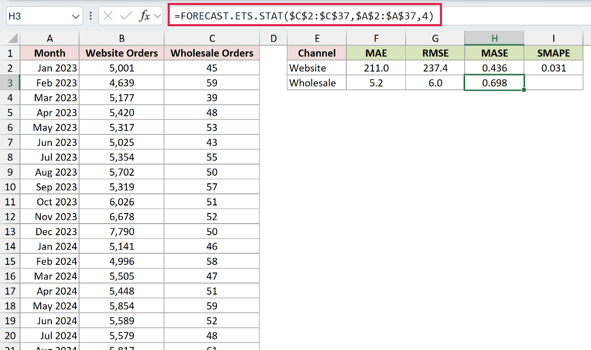
Wholesale MASE is 0.698, higher than the website’s 0.436. Both beat their naive benchmarks, but the website has the lower scaled error.

Finally, calculate wholesale SMAPE in I3:

=FORECAST.ETS.STAT($C$2:$C$37,$A$2:$A$37,5)

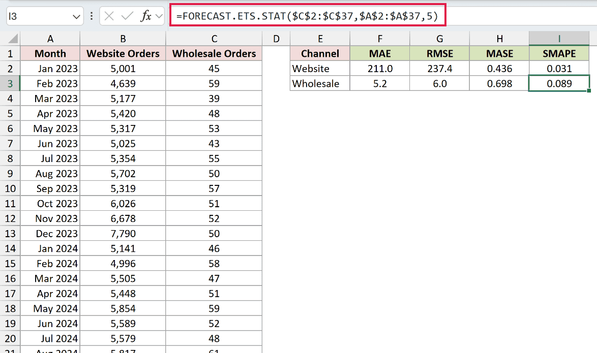
Wholesale SMAPE is 0.089, also higher than the website’s 0.031.

MAE and RMSE help you understand the miss in orders. MASE and SMAPE remove the volume scale, making the comparison across channels more useful.

Example 6: Expose a Bad Missing-Month Assumption

A missing winter reading doesn’t mean the household stopped using gas.

Below is the dataset. A:B contain monthly gas usage; Nov 2024 is followed by Jan 2025, so the missing month is absent from the timeline.

The D:G panel contains data-completion settings and labeled spaces for MAE, RMSE, and MASE. The zero-completion row will demonstrate the mistake.

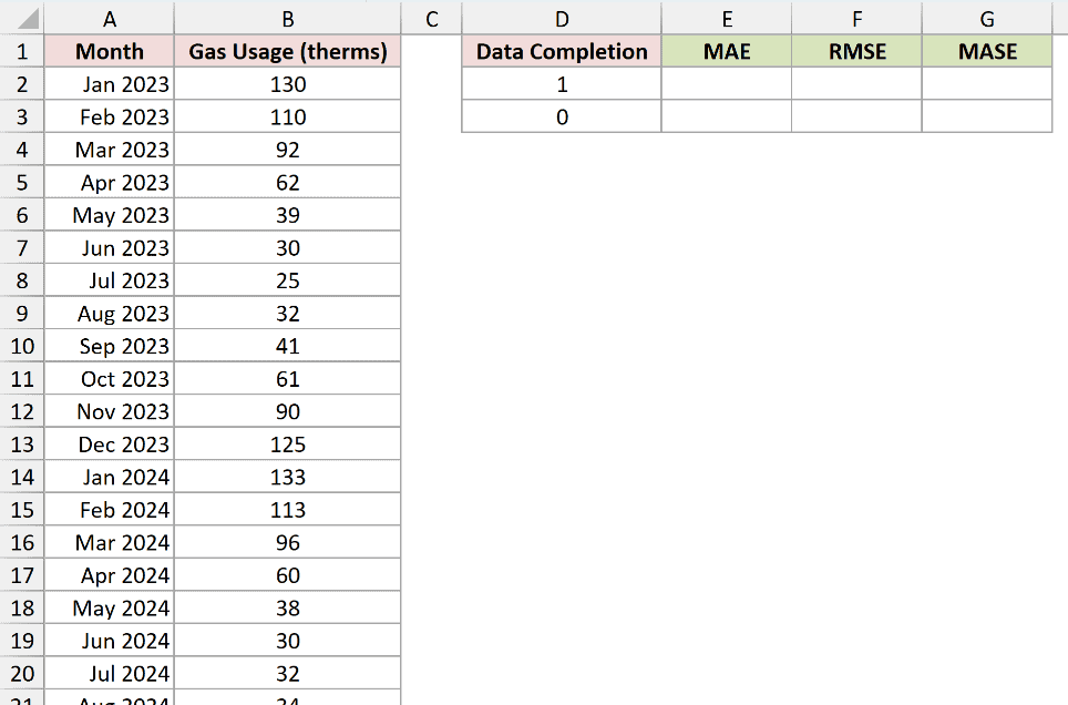
We want to measure how treating the missing month as zero harms the model’s fit.

Enter MAE in E2 and copy it down to E3:

=FORECAST.ETS.STAT($B$2:$B$36,$A$2:$A$36,6,12,D2)

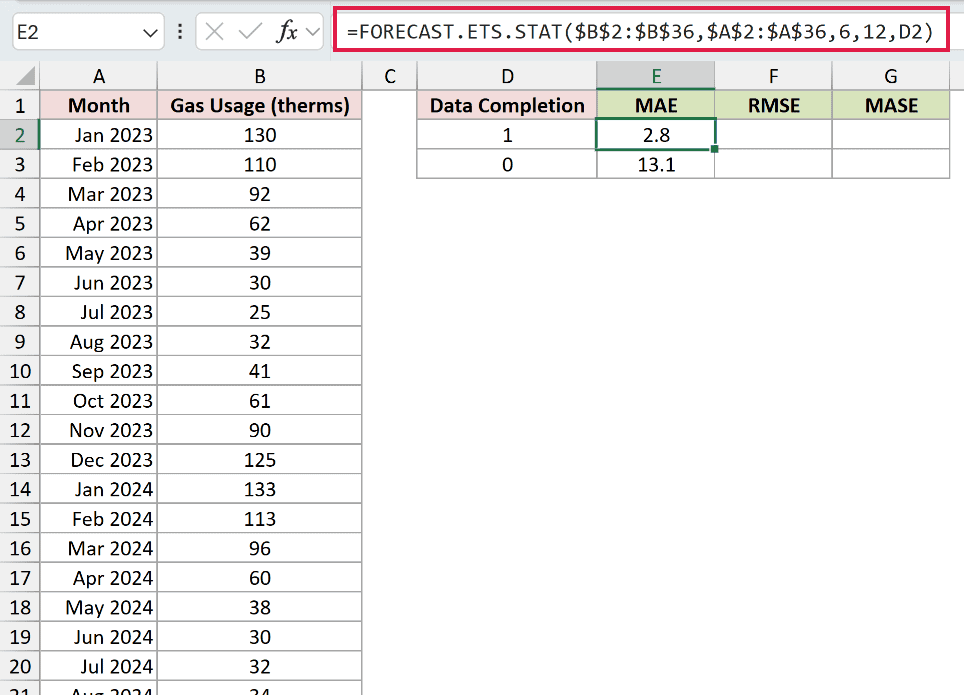
The correct completion setting in row 2 returns 2.8 therms. The zero-completion mistake in row 3 raises MAE to 13.1 therms.

Enter RMSE in F2 and copy it down to F3:

=FORECAST.ETS.STAT($B$2:$B$36,$A$2:$A$36,7,12,D2)

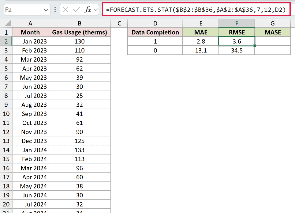
RMSE is 3.6 therms with neighboring-value completion. The zero-completion mistake returns 34.5 therms, exposing the large artificial miss.

Enter MASE in G2 and copy it down to G3:

=FORECAST.ETS.STAT($B$2:$B$36,$A$2:$A$36,4,12,D2)

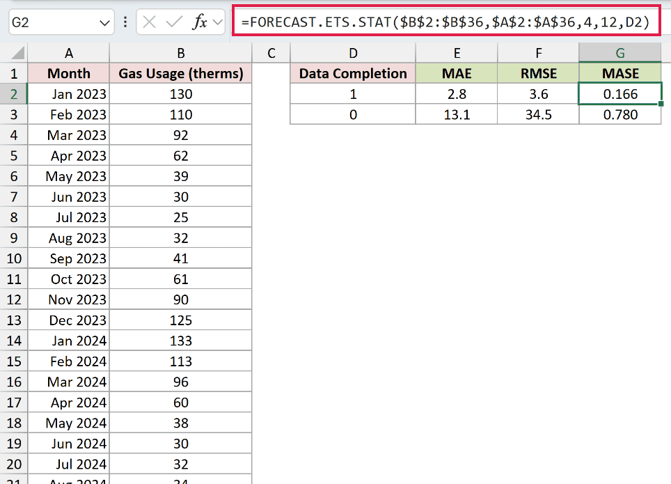
MASE rises from 0.166 to 0.780 in the zero-completion mistake. That wrong assumption still passes the below-1 check, so the label alone wouldn’t catch it.

The history and 12-month cycle stay fixed; only the data-completion reference changes between rows.

Choose the setting that reflects what happened. Here, a missing reading needs estimation, not an invented zero during a high-usage season.

Tips & Common Mistakes

• Check compatibility. FORECAST.ETS.STAT is available in Excel 2016 and later on the desktop. It isn’t available in Excel for the web, iOS, or Android.
• Keep statistic codes separate from seasonality. The statistic code selects the output; seasonality controls the model. Statistic types 0 and 9 return #NUM!.
• Match the input sizes. Different-sized values and timeline ranges return #N/A. Check the endpoints of both ranges.
• Don’t reject duplicate dates automatically. Excel aggregates duplicate time points using the aggregation argument. Omitted or 1 means AVERAGE; explicit 0 returns #NUM!.
• Keep SMAPE’s scale straight. The returned value is a fraction. Apply percentage formatting if you prefer, without treating the unformatted fraction as a percentage already.
• Read step size in timeline units. Type 8 reports spacing, not a confidence interval or the detected seasonal cycle.
• Allow for changes beyond the history. Lower errors help compare settings, but future changes in demand or usage can still make a forecast miss.

I covered reading statistics, checking a forecast’s fit, comparing seasonality, testing timeline spacing, comparing channels, and spotting a bad missing-month setting.

List of All Excel Functions

Related Excel Functions / Articles:

• FORECAST.LINEAR Function in Excel
• FORECAST Function in Excel
• GROWTH Function in Excel