
Excel’s ASINH function returns the inverse hyperbolic sine of any real number.
It’s useful for compressing wide ranges of positive and negative values. Unlike a regular logarithm, ASINH keeps negative values and maps zero to zero.
In this article, I’ll show you how to transform signed data, compare ASINH with LN, and choose a useful scale.
ASINH Function Syntax in Excel
The ASINH function takes one numeric argument.
=ASINH(number)
- number (required) is any real number whose inverse hyperbolic sine you want to calculate.
When to Use ASINH Function
- Compress a wide range of signed profit, loss, or cash flow values.
- Reverse a SINH result and return to the original number.
- Scale values before transforming them so comparisons use consistent units.
- Avoid precision problems in the expanded LN calculation for large negative numbers.
Example 1: Calculate and Reverse ASINH Values
Let’s start with numbers spanning negative, zero, and positive values.
Below is the dataset. Column A holds the numbers from -1000 to 1000.
The green headers ASINH Result (B1) and Back with SINH (C1) sit above empty bordered cells.
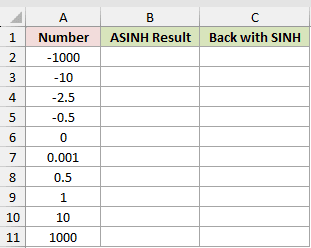
First, we want column B to return the ASINH result for every number.
Here is the formula entered in B2:
=ASINH(A2:A11)
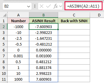
The formula spills ten results down column B. It returns -7.600903 for -1000, 0.000000 for zero, and 7.600903 for 1000.
Next, we want column C to pass those results through SINH and recover the original numbers.
Here is the formula entered in C2:
=SINH(B2:B11)
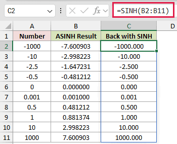
SINH reverses the ASINH calculation. The first and last results return -1000.000 and 1000.000, matching the original values.
Near zero, ASINH stays close to the input. The value 0.001 returns 0.001000.
Large inputs compress sharply. For example, 1000 returns only 7.600903.
All range formulas in this article spill in Excel 2021, Excel 2024, and Microsoft 365.
In Excel 2019 and earlier, enter the first-row formula, such as =ASINH(A2), and fill it down.
Pro Tip: Keep the cells below the formula empty. Any obstruction in the intended result area causes a #SPILL! error.
Example 2: Transform Monthly Profit and Loss
Here’s a practical way to compress monthly results that vary widely.
Below is the dataset. Column A contains Month, and column B contains Net Profit.
The green ASINH Profit header sits above empty bordered cells in column C.
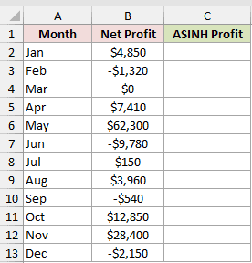
We want column C to transform all twelve monthly profit and loss values.
Here is the formula entered in C2:
=ASINH(B2:B13)
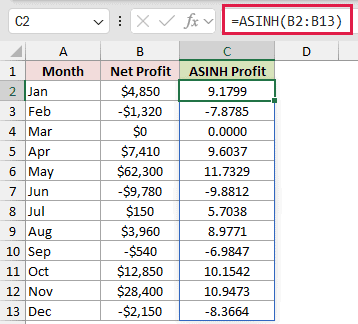
The formula keeps profitable months positive, loss months negative, and the zero month at 0.0000.
May’s $62,300 becomes 11.7329, while June’s -$9,780 becomes -9.8812. This makes a wide signed range easier to compare without discarding losses.
The scale still depends on the units in the source column. Example 4 shows how to control that effect instead of accepting the raw dollar scale.
Example 3: Compare ASINH With LN
Now let’s compare ASINH with the natural logarithm on signed investment results.
Below is the dataset. It lists nine holdings and their Realized Gain/Loss values.
The green LN Result and ASINH Result headers sit above empty bordered cells.
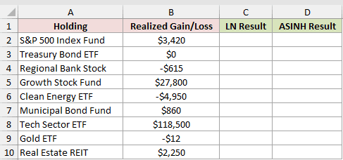
First, we want column C to calculate LN for every gain or loss.
Here is the formula entered in C2:
=LN(B2:B10)
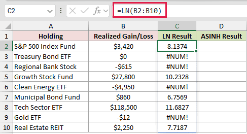
Next, we want column D to apply ASINH to the same values.
Here is the formula entered in D2:
=ASINH(B2:B10)
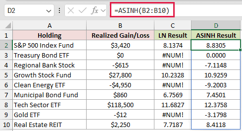
LN returns #NUM! for the zero and negative amounts. ASINH returns a numeric result for every row and keeps each loss negative.
For the positive amounts in this dataset, each ASINH result is about 0.6931 higher than its LN result.
For example, the $3,420 gain returns 8.1374 with LN and 8.8305 with ASINH. The difference comes from ASINH approaching LN of twice the input.
Example 4: Scale Cash Flow Before ASINH
Let’s improve the transformation by choosing a meaningful input scale.
Below is the dataset. Column A contains Week Of dates, and column B contains Net Cash Flow.
The green Scaled ASINH header sits above empty bordered cells in column C. The Scale ($) card in E1:E2 already holds $1,000.
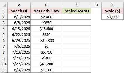
We want column C to divide each cash flow by the fixed scale before applying ASINH.
Here is the formula entered in C2:
=ASINH(B2:B11/$E$2)
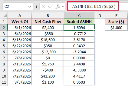
The single reference to the $1,000 scale card in E2 divides all ten cash flow values before ASINH.
A $350 cash flow returns 0.3432, and -$400 returns -0.3900. These smaller values stay close to their scaled inputs of 0.35 and -0.40.
Larger values compress more strongly. The $41,200 week returns 4.4117, while the -$12,300 week returns -3.2044.
Choose a scale that makes sense for the data, then keep it consistent when comparing periods or groups.
Example 5: Avoid LN Formula Precision Loss
The final example compares ASINH with its expanded mathematical expression.
Below is the dataset. Column A contains positive and negative values.
The green ASINH Result and LN Formula Result headers sit above empty bordered cells.
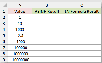
First, we want column B to calculate the result directly with ASINH.
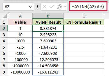
Here is the formula entered in B2:
=ASINH(A2:A9)
Next, we want column C to calculate the same expression with LN and SQRT.
Here is the formula entered in C2:
=LN(A2:A9+SQRT(A2:A9^2+1))
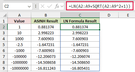
The displayed results match through six decimals for the smaller values, including 1, 10, 1000, -2.5, and -1000.
The manual expression begins drifting for larger negative values. At -10,000,000, ASINH returns -16.811243, while the LN expression returns -16.805431.
This happens because the LN expression adds a large negative number to a nearly equal positive square root. That cancellation loses precision.
Use ASINH directly when accuracy matters. The shorter formula also makes the worksheet easier to read.
Tips & Common Mistakes
- Don’t confuse ASINH with ASIN. ASINH accepts any real number, while
=ASIN(2)returns#NUM!because ASIN only accepts values from -1 through 1. - Check blank source cells before transforming data. ASINH treats a blank cell as zero, so missing data can look like a genuine zero result.
- Numeric text and logical values are coerced. Text
"2"returns 1.443635, and TRUE returns 0.881374. Nonnumeric text such as"abc"returns#VALUE!. - Scale signed business data deliberately. Changing dollars to thousands changes the transformed numbers, so use one scale for values you intend to compare.
LN fails at zero and negative inputs, while ASINH keeps both usable.
Choose one scale for comparable data, and use ASINH directly to avoid the drift shown at -10,000,000.
Other Excel articles you may also like:
