
The DETECTLANGUAGE function in Excel identifies the language of a text value and returns the corresponding code from Microsoft’s online language service.
That code can drive filtering, summaries, quality checks, or another language function. Because the result comes from an online service, Excel needs an internet connection.
In this article, I’ll show you how to turn detected codes into readable names, filter multilingual records, and catch language mismatches before they reach customers.
DETECTLANGUAGE Function Syntax in Excel
DETECTLANGUAGE takes the text you want Excel to evaluate.
=DETECTLANGUAGE(text)
- text (required) is the text to evaluate or a reference to a cell containing that text.
When to Use DETECTLANGUAGE Function
- Identify the language used in customer messages, survey comments, or support requests.
- Convert language codes into readable language names with a lookup table.
- Filter or count records by their detected language.
- Compare localized text with the language expected for each market.
- Choose a target language for an automatic reply or another translation task.
Example 1: Detect Languages in a Column
Let’s start with a list of hotel requests written in different languages.
Below is the dataset. It has room numbers and guest requests, while the empty Language Code column will hold the results.
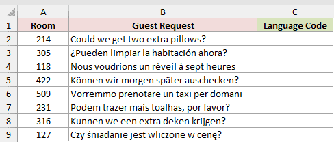
We want one formula to identify the language used in every guest request.
Here is the formula:
=DETECTLANGUAGE(B2:B9)
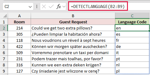
DETECTLANGUAGE reads the range in column B and spills one code per request into column C.
At the time of writing, Microsoft’s service returned en, es, fr, de, it, pt, nl, and pl for the requests.
DETECTLANGUAGE is available in Microsoft 365 for Windows, Mac, and Excel Mobile. It needs an internet connection, and perpetual Excel versions return #NAME?.
Example 2: Convert Codes to Language Names
The returned codes are useful for formulas, but readable names work better in a report.
Below is the dataset. It has customer notes, an empty Language result column, and a code lookup table for readable names.
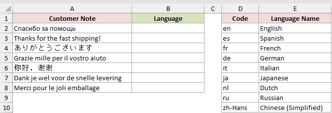
We want to detect each note and return its full language name.
Here is the formula:
=XLOOKUP(DETECTLANGUAGE(A2:A8),D2:D10,E2:E10,"Not in list")
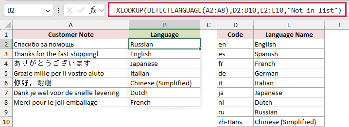
DETECTLANGUAGE creates the lookup values. XLOOKUP matches those codes in column D and returns the names from column E.
The fourth argument returns Not in list instead of #N/A when a detected code is missing from D2:D10. At the time of writing, all seven notes matched.
At the time of writing, the results were Russian, English, Japanese, Italian, Chinese (Simplified), Dutch, and French.
Most returned codes are two letters, but not all. zh-Hans carries a script subtag after the language code, so D2:D10 must hold the exact code the service returns.
Example 3: Filter Non-English Text
Here’s a quick way to separate return reasons that need another language workflow.
Below is the dataset. Column A holds return reasons. Column C has its own Return Reason header above the empty result cells.
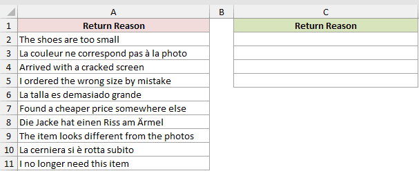
We want to return only the reasons that DETECTLANGUAGE does not classify as English.
Here is the formula:
=FILTER(A2:A11,DETECTLANGUAGE(A2:A11)<>"en")
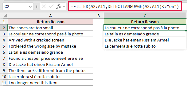
The comparison creates TRUE for every detected code other than en. FILTER returns the matching text from column A.
At the time of writing, the first returned reason was La couleur ne correspond pas à la photo, followed by La talla es demasiado grande.
The remaining results were Die Jacke hat einen Riss am Ärmel and La cerniera si è rotta subito.
FILTER is available in Excel 2021 and later, but this combined formula still needs Microsoft 365 because it uses DETECTLANGUAGE.
Example 4: Count Questions by Language
You can detect a list once, then reuse those codes in a summary.
Below is the dataset. Column A holds webinar questions, column B will hold detected codes, and column E will hold counts for the codes listed in D.
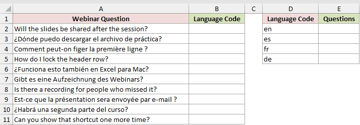
First, we want to create a helper spill containing the language code for each question.
Here is the helper formula:
=DETECTLANGUAGE(A2:A11)
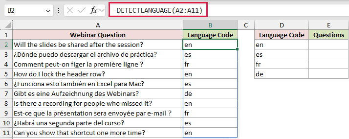
At the time of writing, the helper column identified questions using en, es, fr, and de.
Next, we want to count how often each code appears in that spill.
Here is the counting formula:
=COUNTIF(B2#,D2:D5)
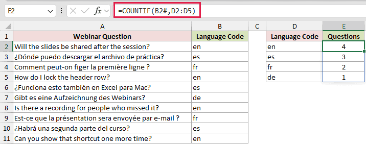
The spill reference B2# passes the existing helper results to COUNTIF. DETECTLANGUAGE runs once per question instead of making another service request for the summary.
At the time of writing, COUNTIF returned 4 for en, 3 for es, 2 for fr, and 1 for de.
Example 5: Catch the Wrong Language
Now let’s check localized email subjects before they are sent.
Below is the dataset. It has each market, its expected code, a welcome email subject, and an empty Language Check result column.
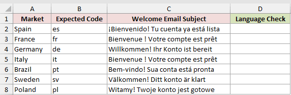
We want to compare each detected language with the expected code for that market.
Here is the formula:
=IF(DETECTLANGUAGE(C2:C8)=B2:B8,"OK","Wrong language")
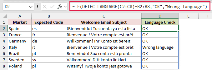
The detected codes for C2:C8 are compared row by row with the Expected Code values in B2:B8.
The OK and Wrong language results spill into D2:D8.
At the time of writing, every correctly localized row returned OK. The Italy row returned Wrong language because a French subject was pasted there.
That Italy result is the finding this check exists to catch. It is not an Excel error or another valid language option.
Example 6: Reply in the Sender’s Language
Finally, DETECTLANGUAGE can choose the target language for an automatic reply.
Below is the dataset. It has contact form messages, an empty Auto-Reply column, and an English reply template in the card on the right.

We want to translate the fixed English template into the language detected for each incoming message.
Here is the formula:
=TRANSLATE(D2,"en",DETECTLANGUAGE(A2:A7))
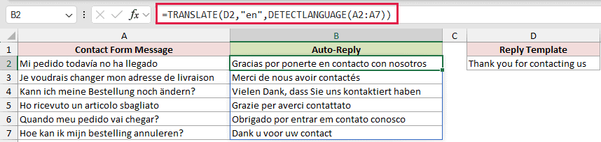
The second argument identifies the template as English.
Inside the formula, DETECTLANGUAGE returns one target-language code per message as TRANSLATE’s third argument. The six translated replies spill into B2:B7.
At the time of writing, the Spanish and French replies were Gracias por ponerte en contacto con nosotros and Merci de nous avoir contactés.
The German and Italian replies were Vielen Dank, dass Sie uns kontaktiert haben and Grazie per averci contattato.
The Portuguese and Dutch replies were Obrigado por entrar em contato conosco and Dank u voor uw contact.
Microsoft’s service may return different wording later. In testing, an English message returned the unchanged English template when the source and target languages matched.
For fixed approved wording, keep human-written replies in a lookup table instead of translating a template each time.
Tips & Common Mistakes
- A truly blank cell or
""returns an empty result. A blank inside a spilled range also leaves that result row empty without stopping the other detections. - Numeric input can still receive a language guess. In testing,
12345returneden, so exclude IDs and other number-only cells from language checks. - Short text is unreliable. In testing,
OKreturneden, whileSireturnediteven though it was intended as Spanish. - Mixed-language text returns one dominant language. At the time of writing,
Thank you, merci beaucoupreturnedfr, not the language used first. - DETECTLANGUAGE and TRANSLATE use an online service, so their results can change. A temporary
#BUSY!state can appear while Excel waits for a response. - A very long cell can trigger Text Too Long, and exceeding the daily request quota can trigger Request Throttled. Either prevents a code from returning.
- TRANSLATE can detect an omitted source language itself. You do not need DETECTLANGUAGE merely to translate text into English unless you also need the code.
- Keep spill cells clear. Blocking content causes
#SPILL!, and no codes appear until that content is cleared.
Treat DETECTLANGUAGE as a starting point, not a guarantee.
Test it with your real text before you build the next step around its codes.
Related Excel Functions / Articles:
