
The SUMX2PY2 function in Excel squares the values in each corresponding pair, adds those squares, and returns the total across all pairs.
This is useful when positive and negative measurement errors shouldn’t cancel each other out. Squaring preserves their size while removing their signs.
If either cell contains text or is blank, Excel skips the entire pair, including the number on the other side.
I’ll show you how to total squared measurements, calculate combined tolerances, and spot the effect of incomplete pairs.
SUMX2PY2 Function Syntax in Excel
SUMX2PY2 takes the following required arguments:
=SUMX2PY2(array_x, array_y)
- array_x is the first set of values. You can supply a range, an array, or a single number.
- array_y is the second set of values, with the same number of positions as the first.
Excel squares each value separately before adding. It doesn’t add the paired values first and then square their sum.
When to Use SUMX2PY2 Function
- Total squared errors across paired measurement columns.
- Calculate a rectangular screen’s diagonal by adding the squared width and height, then taking the square root.
- Combine independent tolerance contributions using a root-sum-square calculation.
- Calculate a combined squared total for a selected group of records.
Example 1: Total Squared Measurement Errors
Let’s start with parts that have both positive and negative measurement errors.
Below is the dataset. Columns B and C contain width and length errors, column D will show each part’s contribution, and F2 will hold the total.
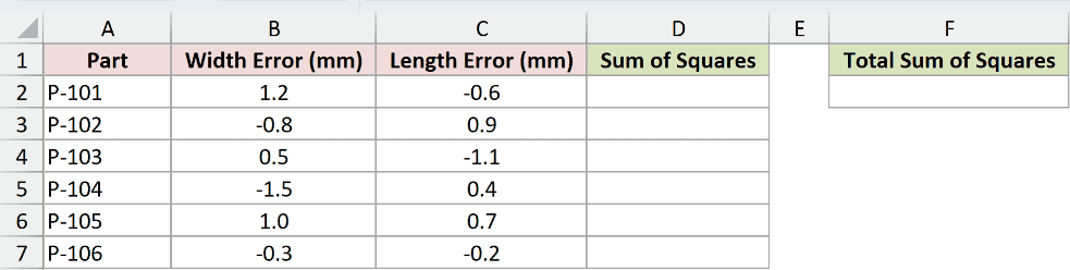
We want the total of the squared width and length errors across all listed parts.
Enter this formula in F2:
=SUMX2PY2(B2:B7,C2:C7)
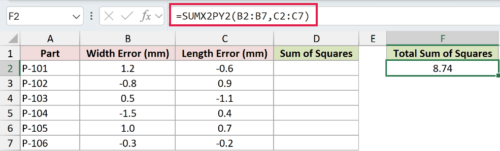
The result is 8.74 square millimeters. SUMX2PY2 returns a single total from the ranges, so it doesn’t spill a separate answer for each part.
To see the contributions behind that total, enter this helper formula in D2:
=B2:B7^2+C2:C7^2
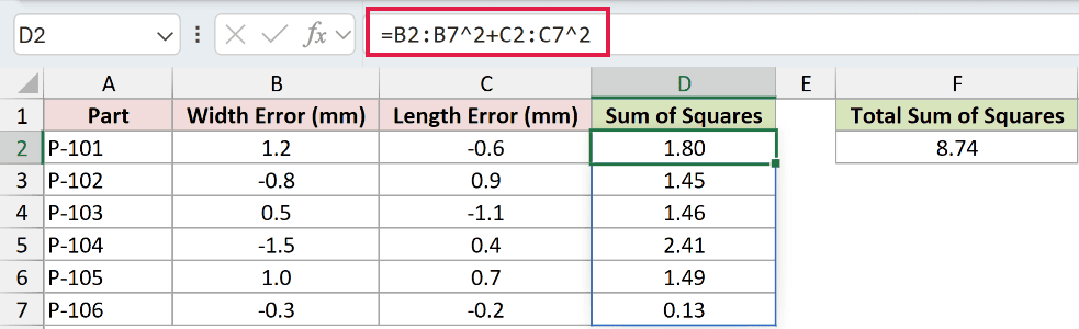
The helper spills into D2:D7. Its results are 1.80, 1.45, 1.46, 2.41, 1.49, and 0.13, which together make the total.
For P-101, the inputs are 1.2 and -0.6. Squaring each separately produces the positive contribution shown as 1.80.
This helper spills in Excel 2021, Excel 2024, and Microsoft 365. In Excel 2019 and earlier, calculate each row’s squared contribution separately and copy down.
Example 2: Calculate a Screen Diagonal
You can also pass SUMX2PY2 a single pair of cells.
Below is the dataset. Columns B and C contain screen widths and heights in inches, and column D is reserved for the diagonals.
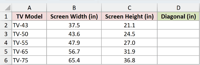
We want to calculate the diagonal of each rectangular screen from its width and height.
SQRT returns a square root, so wrapping it around SUMX2PY2 converts the sum of squared dimensions into a diagonal length.
Enter this formula in D2, then copy it down through D6:
=SQRT(SUMX2PY2(B2,C2))
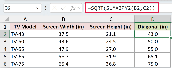
The first screen’s width of 37.5 inches and height of 21.1 inches produce a diagonal displayed as 43.0 inches.
The remaining diagonals display as 50.0, 55.0, 65.1, and 75.0 inches.
We copy this formula down because each screen needs its own result. Passing the full columns to SUMX2PY2 would combine every screen into a single calculation.
Example 3: Combine Tolerance Contributions
Now let’s combine machining and positioning tolerances for an assembly.
Below is the dataset. Columns B and C contain tolerance magnitudes, while the card in E:F has labeled cells for combined tolerance and a worst-case comparison.

We want a root-sum-square estimate, then a comparison showing what happens when all tolerances add in the same direction.
SQRT takes the square root of SUMX2PY2’s total, converting square millimeters back to millimeters. Enter this formula in F2:
=SQRT(SUMX2PY2(B2:B6,C2:C6))
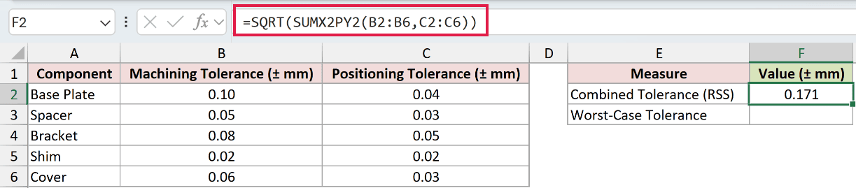
The combined tolerance displays as 0.171, interpreted as ±0.171 mm in this example. RSS means root sum square: square the contributions, add them, then take the square root.
For the worst-case comparison, SUM adds all the listed tolerance magnitudes without squaring. Enter this formula in F3:
=SUM(B2:C6)
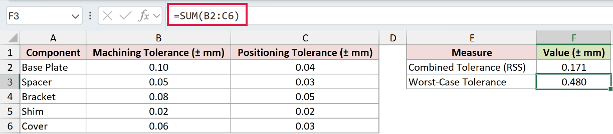
The worst-case comparison displays 0.480, or ±0.480 mm. This assumes every contribution reaches its limit in the same direction.
Pro Tip: Treat RSS as an estimate under an independent-error model, not a guaranteed maximum. The tolerance inputs need a consistent statistical basis; SUMX2PY2 doesn’t check that assumption.
Example 4: Calculate Tolerance for Each Kit
A mixed parts list needs a separate calculation for each kit.
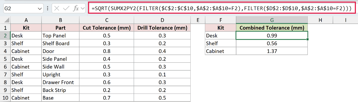
Below is the dataset. Columns A:D list kits, parts, and tolerances. F2:F4 contains the kit names, and column G will hold their combined tolerances.
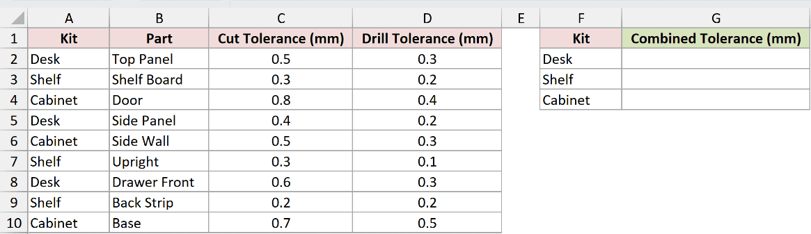
We want to combine only the tolerance contributions belonging to the kit named on each summary row.
FILTER selects matching rows before SUMX2PY2 squares and totals their values. SQRT then takes the square root to return the combined tolerance in millimeters.
Enter this formula in G2 and copy it down through G4:
=SQRT(SUMX2PY2(FILTER($C$2:$C$10,$A$2:$A$10=F2),FILTER($D$2:$D$10,$A$2:$A$10=F2)))
How this formula works:
- The first FILTER selects cut tolerances for the kit named in F2.
- The second FILTER selects drill tolerances using the same condition, keeping the pairs aligned.
- SUMX2PY2 combines the squared values, and SQRT converts that total into an RSS tolerance.
- The dollar signs keep the source ranges fixed as the kit reference changes during fill-down.
The results display as 0.99 mm for Desk, 0.56 mm for Shelf, and 1.37 mm for Cabinet.
FILTER requires Excel 2021 or later. Although it creates arrays inside this formula, SUMX2PY2 combines them into a single result for each kit.
Example 5: Recover the Squared Score Differences
Two judges have scored the same entries. Let’s use their scores to calculate the total squared disagreement.
Below is the dataset. Columns B and C hold the judges’ scores, and the Measure/Value card has labeled rows for the total and comparison calculations.
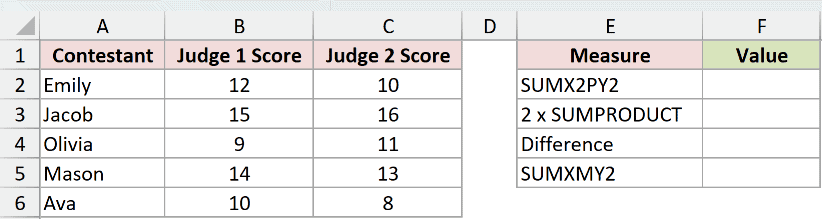
We want to start with the squared-score total and use it to calculate the judges’ total squared disagreement.
First, enter SUMX2PY2 in F2:
=SUMX2PY2(B2:B6,C2:C6)
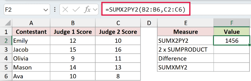
The result is 1456, the combined total of both judges’ squared scores.
SUMPRODUCT multiplies corresponding scores and adds those products. We need twice that amount to remove the shared product term from the squared-score total.
Enter this supporting formula in F3:
=2*SUMPRODUCT(B2:B6,C2:C6)
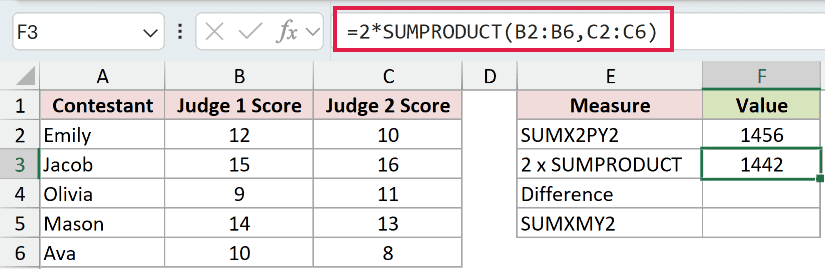
That supporting calculation returns 1442. Subtract it from the SUMX2PY2 total in F4:
=F2-F3
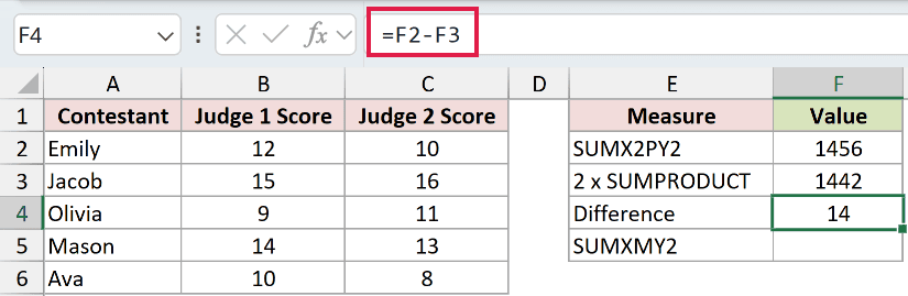
The result is 14. Subtracting twice the paired products turns the sum of the separate squares into the sum of squared differences.
SUMXMY2 calculates those squared differences directly. Use it in F5 as a comparison check on the calculation we built from SUMX2PY2:
=SUMXMY2(B2:B6,C2:C6)
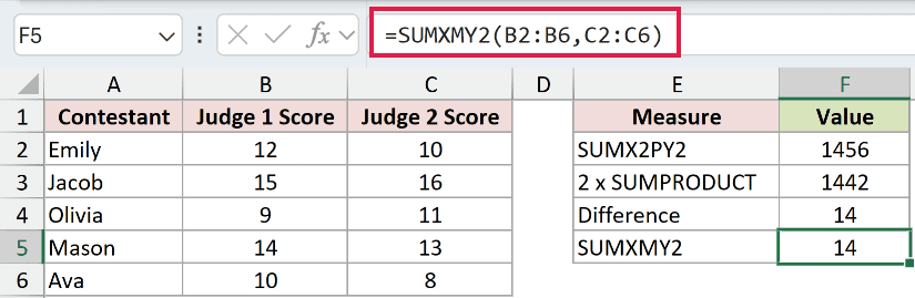
The comparison also returns 14. It confirms the relationship, while showing why the original SUMX2PY2 total isn’t itself a measure of disagreement.
Example 6: See Why Incomplete Pairs Disappear
Missing readings change which numbers SUMX2PY2 includes.
Below is the dataset. Columns B and C contain vibration readings, including an Offline entry and a blank. The card has rows for complete-pair and every-number comparisons.
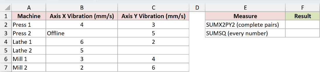
We want the sum of squared readings from machines that have numeric readings on both axes.
Enter this formula in F2:
=SUMX2PY2(B2:B7,C2:C7)
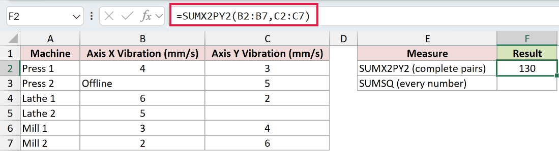
SUMX2PY2 returns 130. It skips Press 2 because B3 contains Offline, and Lathe 2 because C5 is blank.
That means the numeric reading of 5 in C3 is excluded too. So is the numeric reading of 5 in B5.
For comparison, SUMSQ squares and adds every numeric value independently. It doesn’t require a numeric partner, which makes it useful for seeing what SUMX2PY2 excluded.
Enter this comparison formula in F3:
=SUMSQ(B2:B7,C2:C7)
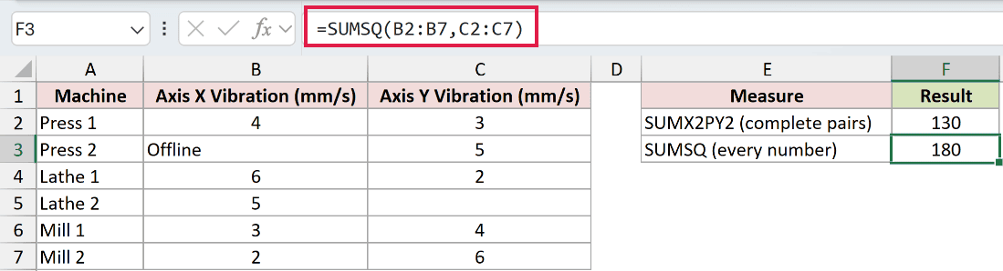
The SUMSQ comparison returns 180 because it includes the unpaired numeric readings.
Pro Tip: Don’t replace missing readings with zero merely to keep a pair in the calculation. A zero says the reading was measured as zero; a blank says it is missing.
Tips & Common Mistakes
- Match the range sizes. Different numbers of positions return
#N/A. Check both the starting and ending rows. - Keep related records aligned. Excel pairs by position, not by the labels beside the values. Sorting only one input column breaks that relationship.
- Check for complete numeric pairs. If none remain, SUMX2PY2 returns
#DIV/0!, even though your formula doesn’t contain division. - Watch numbers stored as text. They cause their pairs to be skipped. Quoted numeric text supplied directly is skipped too; it isn’t converted into a number.
- Logical values aren’t numeric readings here. TRUE and FALSE cause the corresponding pair to be skipped, just like text or a blank.
- Zeros are valid inputs. A numeric zero keeps its pair eligible, provided the other value is numeric too.
Other Excel articles you may also like:
