
Excel’s SUMXMY2 function returns the sum of squared differences between corresponding values in two arrays.
It pairs the first value with the first, the second with the second, and so on.
Squaring removes negative signs and makes larger gaps contribute more to the total. The function returns one value, and both arrays must contain the same number of corresponding elements.
In this article, I’ll show you how to measure forecast error, calculate coordinate distance, preserve pairings after filtering or lookup, and compare matching matrices.
SUMXMY2 Function Syntax in Excel
The SUMXMY2 function uses the following syntax:
=SUMXMY2(array_x,array_y)
array_xis the first required array or range of values.array_yis the second required array or range. Its values are paired position by position witharray_x.
SUMXMY2 returns #N/A when the arrays contain different numbers of values.
When to Use SUMXMY2 Function
- Measure total squared error between actual and forecast values.
- Calculate squared distance between matching coordinate arrays.
- Compare selected rows after filtering two paired columns with the same condition.
- Compare shuffled datasets after aligning both arrays by a shared key.
- Measure total squared difference across two equally shaped matrices.
Example 1: Calculate Total Squared Forecast Error
Let’s begin with product forecasts and actual sales.
Below is the dataset with six products, their actual units, forecast units, and empty columns for row contributions and the total.
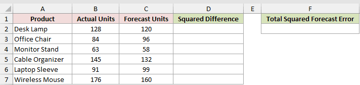
We first want to see how much each product contributes to the total squared error.
Enter this formula in cell D2:
=(B2:B7-C2:C7)^2
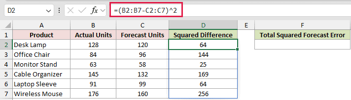
In Excel 2021, Excel 2024, and Microsoft 365, the formula spills the six squared differences through D7.
The Desk Lamp difference is 8 units, so its contribution is 64. The Wireless Mouse difference is 16 units, giving the largest contribution of 256.
We now want one total for all six product differences.
Enter this SUMXMY2 formula in cell F2:
=SUMXMY2(B2:B7,C2:C7)
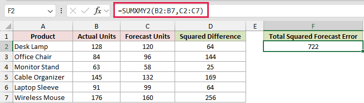
SUMXMY2 subtracts each forecast from its corresponding actual value, squares each difference, and adds the six results. The total squared forecast error is 722.
This total preserves the effect of larger misses. It does not show whether forecasts were generally high or low because squaring removes the direction of each error.
Pro Tip: SUMXMY2 returns a total. Keep the row-level squared differences when you also need to identify which records contribute most to that total.
Example 2: Calculate Distance Between Coordinates
This example turns a squared difference into a distance.
Below is the dataset with X and Y coordinates for a reference warehouse position and a new position.
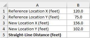
We want to calculate the straight-line distance between the two positions in feet.
Enter this formula in cell B5:
=SQRT(SUMXMY2(B1:B2,B3:B4))
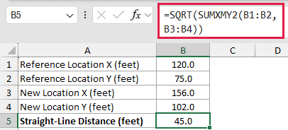
SUMXMY2 pairs the two X coordinates and the two Y coordinates. Their squared differences are 1,296 and 729, totaling 2,025.
The SQRT function converts that squared distance back to the original unit. The result is 45.0 feet.
Order still matters inside each array. Pairing an X coordinate with a Y coordinate would calculate a different and meaningless distance.
Example 3: Error for Filtered Paired Data
Now let’s calculate squared error for one region.
Below is the dataset with regional actual and forecast orders, plus West selected as the region to analyze.
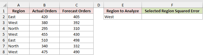
We want to calculate total squared error for the West rows while keeping actual and forecast values aligned.
Enter this formula in cell F2:
=SUMXMY2(FILTER(B2:B8,A2:A8=E2),FILTER(C2:C8,A2:A8=E2))
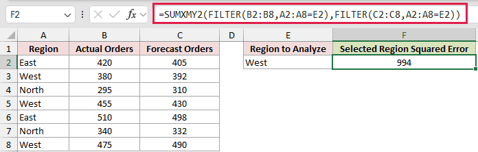
The first FILTER function returns West actual orders. The second returns West forecasts using the identical row mask A2:A8=E2.
Using the same mask keeps the three pairs in matching order. Their squared differences are 144, 625, and 225, which total 994.
SUMXMY2 remains a single-value reducer even though FILTER creates dynamic arrays inside it. The formula returns one result in F2 rather than spilling.
FILTER is available in Excel 2021, Excel 2024, and Microsoft 365. Earlier versions need another method to create the matching subsets.
Pro Tip: Filter both value columns with the same include condition. Different masks can change the array lengths or pair unrelated rows.
Example 4: Align Shuffled Data With XLOOKUP
Here’s a common alignment problem.
Below is the dataset with actual orders in Week 1 to Week 6 order and forecast orders stored in a different week order.
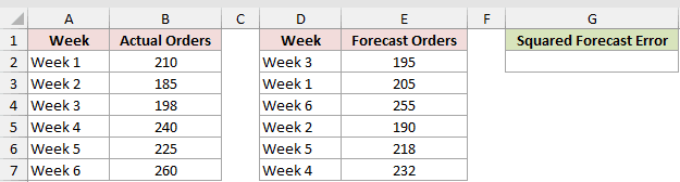
We want to align each forecast with its week before calculating squared forecast error.
Enter this formula in cell G2:
=SUMXMY2(B2:B7,XLOOKUP(A2:A7,D2:D7,E2:E7))
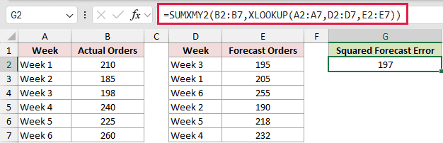
The XLOOKUP function finds each week from A2:A7 in D2:D7 and returns forecasts in the same order as the actual values.
SUMXMY2 then compares the aligned pairs. The six squared differences are 25, 25, 9, 64, 49, and 25, giving a total of 197.
Comparing B2:B7 directly with E2:E7 would pair rows by position rather than week. The formula could calculate successfully while answering the wrong question.
XLOOKUP is available in Excel 2021, Excel 2024, and Microsoft 365. It is not available in Excel 2016 or Excel 2019.
Example 5: Compare Matching Matrices
Let’s finish with two small measurement grids.
Below is the dataset with target and measured readings for three sensors across three tests.

We want to total the squared differences between corresponding cells in the two 3-by-3 matrices.
Enter this formula in cell K2:
=SUMXMY2(B2:D4,G2:I4)

SUMXMY2 pairs B2 with G2, C2 with H2, and continues through D4 and I4. It handles all nine corresponding cells in one calculation.
Sensor A contributes 6, Sensor B contributes 6, and Sensor C contributes 3. The total squared difference is 15.0.
For a matrix comparison, keep the same shape and cell order so corresponding positions hold matching readings. A shifted or transposed matrix changes the pairings.
Tips & Common Mistakes
- Keep the arrays the same size. SUMXMY2 returns
#N/Awhen they contain different numbers of values. - Align records before comparing them. Sorting one range alone or using unrelated row orders pairs the wrong values.
- Text, logical values, and empty cells inside referenced arrays are ignored. Zero values are included.
- Do not confuse SUMXMY2 with SUMX2MY2. SUMXMY2 squares each difference, while SUMX2MY2 subtracts one squared value from another.
- SUMXMY2 returns one result. It can accept arrays produced by dynamic-array functions without spilling the final total.
- A SUMPRODUCT formula can calculate the same metric, but SUMXMY2 states the squared-difference operation directly.
- The row-contribution formula in Example 1 needs empty destination cells. A blocked range produces a
#SPILL!error.
SUMXMY2 adds squared differences across paired arrays. The examples used it for forecast error, coordinate distance, filtered data, keyed records, and matching matrices.
I hope you found this article helpful.
Related Excel Functions / Articles:
