
The VARPA function in Excel calculates population variance, including text and logical values in referenced cells. Variance measures how spread out the values are around their average.
Use it when your list represents the entire group. A label such as “No sales” can count as zero, keeping that person in the calculation.
That same behavior can cause trouble when text represents missing information or an imported number. VARPA can’t tell what the text means.
In this article, I’ll show you how to include zero-sales entries, interpret TRUE/FALSE results, and handle text correctly when calculating variance by group.
VARPA Function Syntax in Excel
The VARPA syntax accepts values or references to the cells you want to measure:
=VARPA(value1,[value2],...)
- value1 (required): The first value or cell range in the population.
- value2, … (optional): Additional values or ranges to include in the same calculation.
For referenced cells, VARPA uses numbers as entered, counts TRUE as 1, and counts FALSE and text as 0. It ignores empty cells.
Population variance averages the squared distances from the population’s mean. Its units are squared, so a variance of sales counts isn’t itself a count of sales.
When to Use VARPA Function
- Measure variation across a complete roster when text labels represent zero activity.
- Calculate variance for a complete TRUE/FALSE checklist.
- See how text and cells that look blank affect population variance.
- Compare groups while keeping zero-activity members in each population.
Example 1: Include Agents With No Sales
Let’s start with an office’s complete agent roster for the quarter.
Below is the dataset. Columns A and B list agents and homes sold, while the labeled cells in D:E provide space for variance and comparison results.
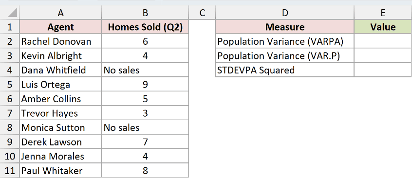
We want population variance for every agent, including those recorded as “No sales.”
Enter this formula in E2:
=VARPA(B2:B11)
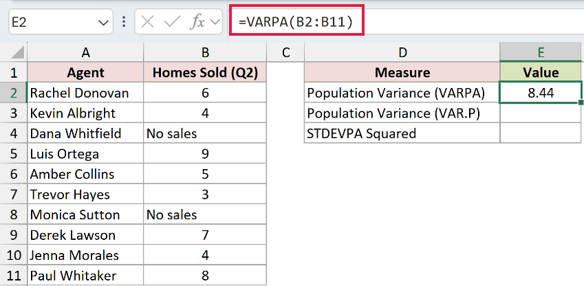
The result is 8.44. VARPA treats Dana Whitfield’s and Monica Sutton’s “No sales” entries as zero, so both agents remain in the population.
VARPA returns a single variance for the entire range. It doesn’t return a separate result for each agent.
For comparison, VAR.P calculates population variance using only numeric cells in a reference. Enter this formula in E3:
=VAR.P(B2:B11)
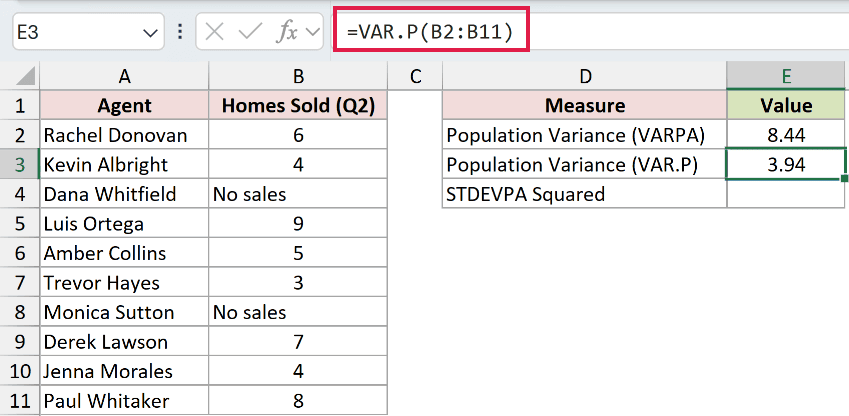
The result in E3 is 3.94 because it excludes the “No sales” entries. That doesn’t describe the complete office roster we’re measuring here.
STDEVPA calculates population standard deviation using the same text and logical-value rules as VARPA. Squaring it lets us check our variance.
Enter the check in E4:
=STDEVPA(B2:B11)^2
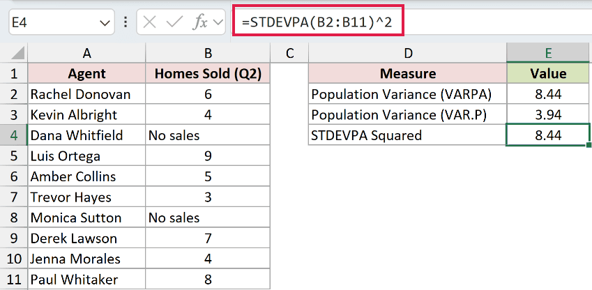
The check returns 8.44, matching VARPA. Standard deviation uses the original units; squaring it gives variance in homes squared.
Pro Tip: Count “No sales” as zero when it means no activity. If it means “report not received,” resolve the missing data first.
Example 2: Distinguish Blanks From Empty Text
Cells that look empty don’t always behave the same way.
Below is the dataset. Columns A:C describe each input and its interpretation, while E:F holds the labeled variance comparison cells. B7 is empty; B9 contains empty text.
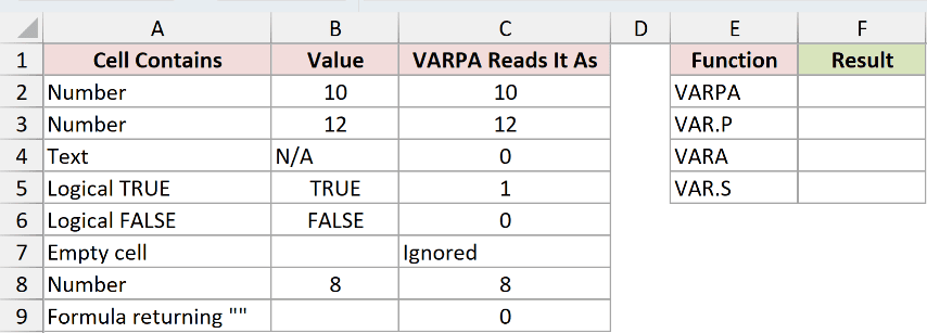
We want to see which entries VARPA includes and how the population and sample comparisons differ.
To reproduce the empty-text input, B9 contains this formula:
=""
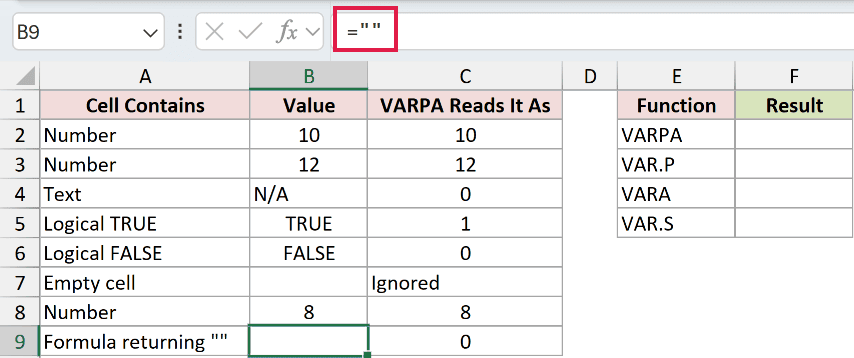
Its displayed result is empty text. This setup cell lets us test how VARPA handles an entry that looks blank.
Enter the VARPA formula in F2:
=VARPA(B2:B9)
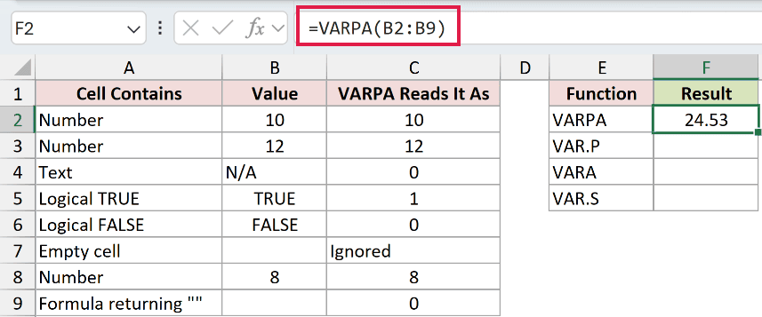
VARPA displays 24.53. It ignores the empty B7 but counts B9’s empty text as 0.
The text “N/A” also counts as 0. It’s a text label in this example, not an Excel error. TRUE contributes 1, and FALSE contributes 0.
For the numeric-only population comparison, VAR.P skips text and logical values in the reference. Enter this in F3:
=VAR.P(B2:B9)
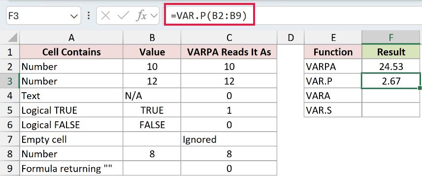
The result in F3 is 2.67. It measures only the numeric entries, so it uses a different population from VARPA.
VARA calculates sample variance while retaining VARPA’s treatment of referenced text and logicals. Enter its formula in F4:
=VARA(B2:B9)
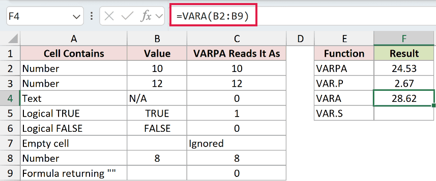
The sample variance is 28.62. It uses a smaller divisor to estimate variance from a sample, rather than describing the entire population.
VAR.S calculates sample variance from numeric cells only. Enter this formula in F5:
=VAR.S(B2:B9)
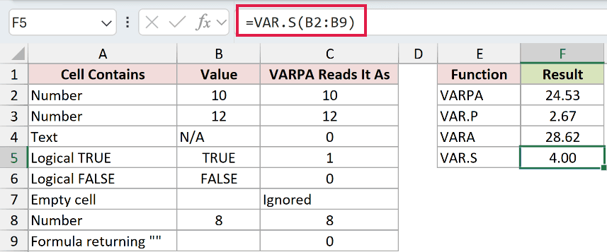
The result in F5 is 4.00. Choose population or sample variance based on your data, then decide whether text and logicals belong in the calculation.
The “N/A” row shows why missing information needs care. Check what the label means before letting VARPA count it as zero.
Example 3: Measure Variation in Pass/Fail Results
A completed smoke-detector checklist gives VARPA a practical use for logical values.
Below is the dataset. Columns A:B list apartments and TRUE/FALSE test outcomes. The measure panel in D:E has labeled cells for variance, pass rate, and a comparison check.
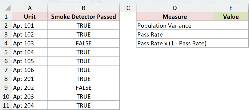
We want variance across the complete checklist, then a pass-rate calculation that helps explain the result.
Enter this formula in E2:
=VARPA(B2:B11)
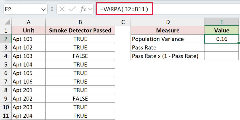
The variance is 0.16. It measures the spread of the recorded pass/fail outcomes. We can also calculate the share of detectors that passed.
To calculate that share, COUNTIF counts TRUE entries and ROWS counts the rows in the complete checklist. Enter this in E3:
=COUNTIF(B2:B11,TRUE)/ROWS(B2:B11)
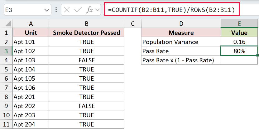
The pass rate is 80%. Every row has a recorded result, so we divide by the full row count.
For a TRUE/FALSE population, multiplying the pass rate by the failure rate checks the variance. Enter this check in E4:
=E3*(1-E3)
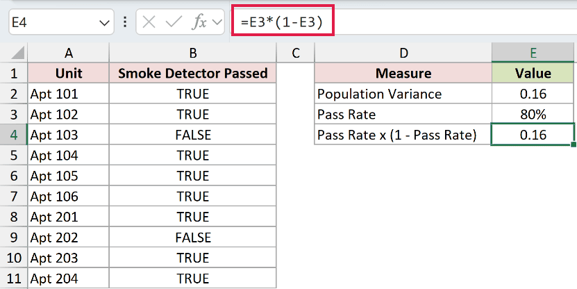
The check returns 0.16, matching VARPA. The formula multiplies the pass rate by its complement, the share that failed.
Keep the pass rate alongside variance when interpreting a checklist. Variance describes variation in outcomes; it doesn’t tell you which outcome is more common.
Example 4: Fix Numbers Stored as Text
An imported number can look correct while VARPA reads it as zero.
Below is the dataset. Columns A:B contain branches and imported loan counts. The measure panel in D:E provides cells for the original results, a text count, and corrected variance.
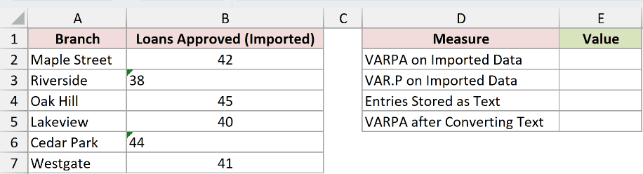
We want variance across all branches using their actual loan counts, including entries imported as text.
First, enter this in E2 to see what goes wrong with the mixed import:
=VARPA(B2:B7)
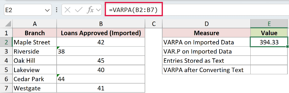
The misleading result is 394.33. Riverside’s “38” and Cedar Park’s “44” are text, so VARPA counts them as zero instead of their intended numbers.
VAR.P calculates population variance from numeric reference cells only. Enter this in E3 to see why skipping text doesn’t fix the import:
=VAR.P(B2:B7)
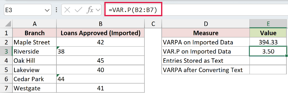
The result in E3 is 3.50. It excludes the text entries, so it still doesn’t describe all branches.
To diagnose the problem, ISTEXT identifies text cells. The double minus converts those checks to numbers, and SUMPRODUCT adds them. Enter this in E4:
=SUMPRODUCT(--ISTEXT(B2:B7))
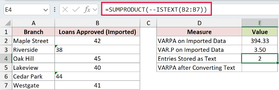
The result is 2, confirming the text entries in the imported column.
Now convert the numeric text before VARPA calculates. Enter this corrected formula in E5:
=VARPA(--B2:B7)
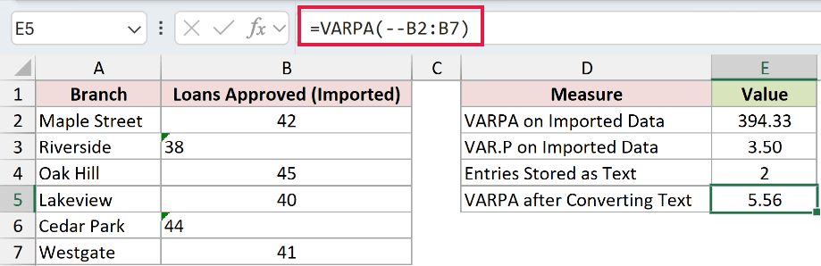
The corrected variance is 5.56. Here, the double minus converts the imported text numbers into actual numbers inside the calculation.
This formula doesn’t change the source cells. For repeated reporting, correct the import process so numeric fields arrive as numbers.
Example 5: Calculate Variance for Each Sales Pod
Filtering a group needs extra care when its text labels represent zero activity.
Below is the dataset. Columns A:C list representatives, pods, and Friday calls. E:G provides pod labels, a FILTER-only mistake column, and a corrected result column.
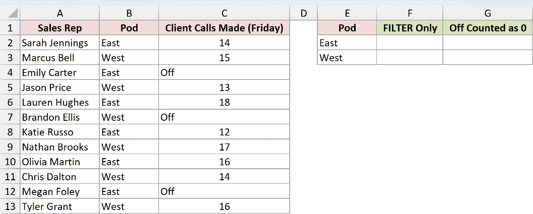
We want each pod’s population variance across its complete roster, including scheduled days off as zero-call days.
FILTER selects entries whose pod matches E2. This example needs Excel 2021, Excel 2024, or Microsoft 365.
Try this in F2 to see the problem, then copy it down to F3:
=VARPA(FILTER($C$2:$C$13,$B$2:$B$13=E2))
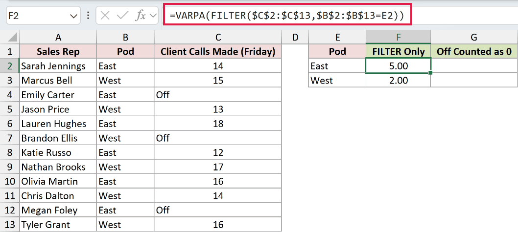
The FILTER-only mistake column displays 5.00 for East and 2.00 for West. VARPA skips the text in this computed array instead of counting it as zero.
That leaves the “Off” representatives out of the calculation, even though our chosen population includes them.
To preserve their zero-call days, ISTEXT identifies text entries and IF replaces them with zero before filtering. Enter the corrected formula in G2:
=VARPA(FILTER(IF(ISTEXT($C$2:$C$13),0,$C$2:$C$13),$B$2:$B$13=E2))
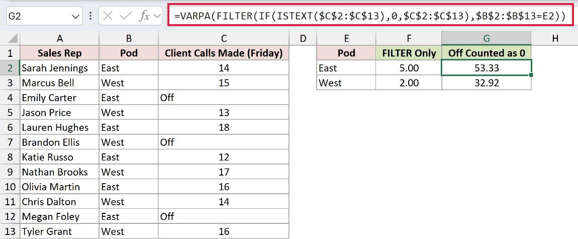
Copy G2 down to G3. The corrected population variances are 53.33 for East and 32.92 for West.
How this formula works:
- ISTEXT identifies the “Off” entries in the calls column.
- IF replaces text with 0 and retains the numeric call counts.
- FILTER selects the converted values for the pod named in E2.
- VARPA calculates a single population variance from those selected values.
The dollar signs keep the source ranges fixed when copying down. E2 changes with the row, selecting the next pod. Copy each formula down to calculate the next pod.
Pro Tip: Count “Off” as zero when those representatives belong in your population. Excluding them measures variation among representatives who worked that day.
Tips & Common Mistakes
- Define the population first. VARPA describes the complete group you provide. A convenient subset isn’t automatically the entire population you intended to measure.
- Don’t confuse empty cells with empty text. A blank cell is ignored, but a formula returning empty text counts as zero in a reference.
- Check what text means. A zero-activity label may belong in the calculation. A note about missing data or a number imported as text needs different treatment.
- Direct arguments follow different text rules. Numeric text typed directly into VARPA is converted to a number. Non-numeric text supplied directly returns
#VALUE!. - A population can contain a single value. VARPA returns 0 because there’s no spread. An all-blank range returns
#DIV/0!because there’s nothing to measure. - VARPA works in every version of Excel.
Other Excel articles you may also like:
