Data Validation in Excel: How to Add, Use, and Remove It

Data validation in Excel lets you control what someone can type into a cell, so a status column doesn’t end up with “Out”, “out”, and “OUT”.

You pick a rule, like a list of choices, a number range, or a date window. Excel then rejects anything that breaks it the moment someone presses Enter.

When the built-in rules can’t express what you need, a custom formula can. Excel accepts the entry only when your formula returns TRUE.

In this article, I’ll show you how to build a drop-down list, limit numbers, dates, and text length, and write custom rules that block duplicates or check a code pattern.

After that, I’ll cover input messages, error alerts, and how to edit, find, and remove rules.

Create a Drop-Down List With Data Validation

Let me show you how to add one to a column.

Method #1: Using the List Rule

A list rule turns a cell into a drop-down, so people pick a value instead of typing it.

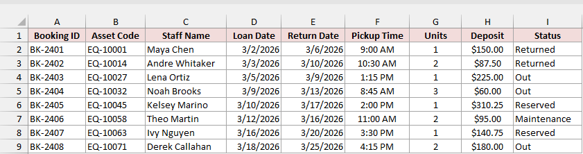
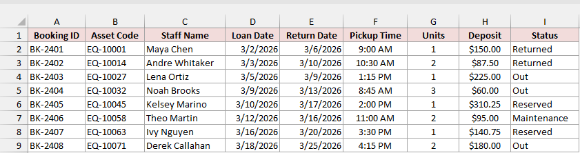
Below I have an equipment Loan Register. I want every Status entry in I2:I9 to be one of four values: Out, Returned, Reserved, or Maintenance.

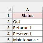
Those four values sit on a separate sheet called Status Choices, in A2:A5.

Here are the steps to add the drop-down:

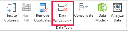
1. Select I2:I9, go to the Data tab, and click Data Validation in the Data Tools group.

2. On the Settings tab, set Allow to List, then enter ='Status Choices'!$A$2:$A$5 in the Source box.

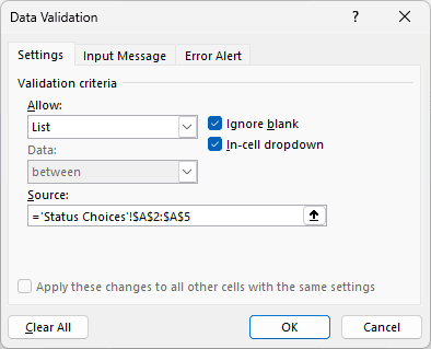
3. Keep In-cell dropdown checked and click OK.

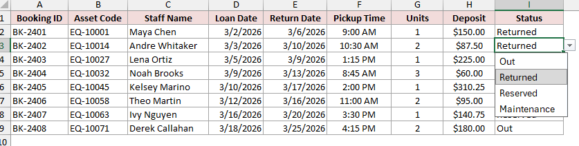
Each Status cell now shows an arrow when you select it, and anything outside the four values gets rejected.

You can also type the items straight into Source, separated by commas (Out,Returned,Reserved,Maintenance).

If you want a drop-down list that updates automatically or depends on another cell, those need a slightly different setup.

Allow Only Certain Numbers, Dates, Times, or Text Lengths

Excel has a built-in rule for each of these. Let me go through them one at a time.

Method #2: Using the Whole Number Rule

If you’re new to data validation, the Whole number rule is a nice place to start.

It accepts whole numbers inside a range and rejects decimals, text, and anything out of bounds.

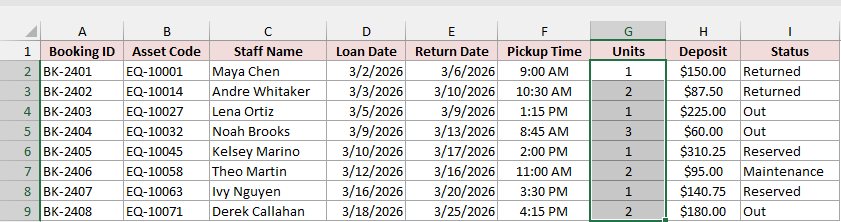
Below I have the same Loan Register. The Units column (G2:G9) records how many units each booking takes, and each booking can take 1 to 5 units.

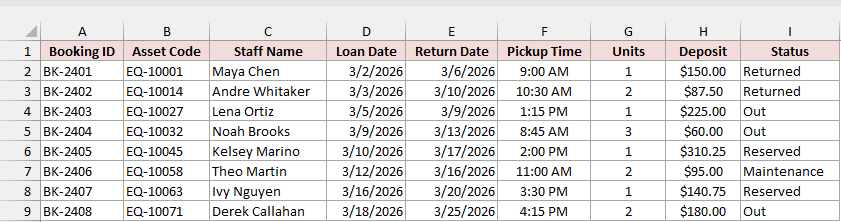
Here are the steps:

1. Select G2:G9 and open Data > Data Validation.

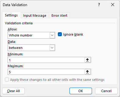
2. Set Allow to Whole number and Data to between. Enter 1 as the Minimum and 5 as the Maximum, then click OK.

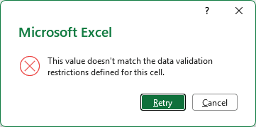
Now try typing 6 into G2. Excel refuses the entry and shows an error alert.

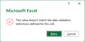
Click Retry to fix the value or Cancel to put back what was there.

The message you see here is Excel’s default one, and I’ll show you how to write your own in Method #11.

Method #3: Using the Decimal Rule

The Decimal rule works like Whole number, except it allows values with decimal places. That makes it the right pick for money, weights, and measurements.

Below I have the Loan Register again. The Deposit column (H2:H9) holds the deposit for each booking, and I want to allow anything from $0 to $500.

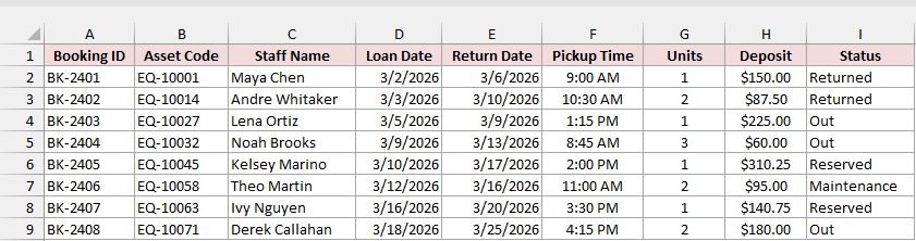
Here are the steps:

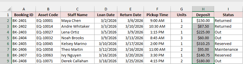
1. Select H2:H9 and open Data > Data Validation.

2. Set Allow to Decimal and Data to between. Enter 0 as the Minimum and 500 as the Maximum, then click OK.

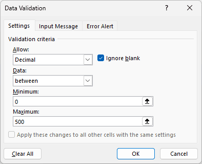
A deposit like $87.50 goes in without a problem. Something like 650 or -20 gets rejected.

Method #4: Using the Date Rule

The Date rule checks that an entry is a real date and that it falls inside the window you set.

It also stops people typing text like “next Tuesday” into a date column.

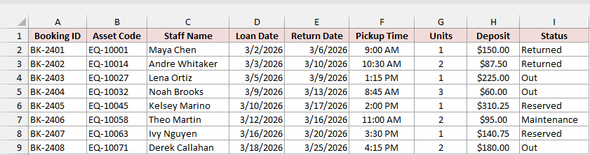
Below I have the Loan Register with Loan Dates in D2:D9. Every loan in this register should be dated sometime in 2026.

Here are the steps:

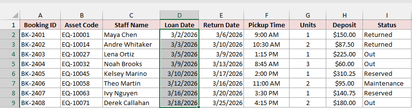
1. Select D2:D9 and open Data > Data Validation.

2. Set Allow to Date and Data to between. Enter 1/1/2026 as the Start date and 12/31/2026 as the End date, then click OK.

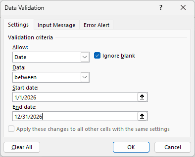
Now 12/31/2025 or 1/1/2027 gets rejected, while any 2026 date goes through.

Note: The date boxes also accept a formula. Set Data to “greater than or equal to” and enter =TODAY() as the Start date, and Excel blocks any date in the past.

Method #5: Using the Time Rule

The Time rule does the same job for times of day. It’s handy for shift logs, appointment slots, and anything tied to opening hours.

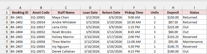
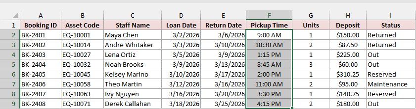
Below I have the Loan Register with Pickup Times in F2:F9. The equipment desk is open from 8:00 AM to 5:00 PM, so pickups should fall inside those hours.

Here are the steps:

1. Select F2:F9 and open Data > Data Validation.

2. Set Allow to Time and Data to between. Enter 8:00 AM as the Start time and 5:00 PM as the End time, then click OK.

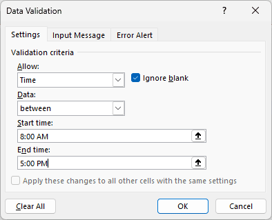
Both ends count as valid, so 8:00 AM and 5:00 PM are accepted. A pickup at 7:30 AM or 5:30 PM gets rejected.

Method #6: Using the Text Length Rule

The Text length rule counts characters instead of checking the value itself.

Use it when an entry has to fit a limit, like a name that prints on a badge or an ID with a fixed length.

Below I have the Loan Register with Staff Names in C2:C9. I want to keep each name to 30 characters or fewer.

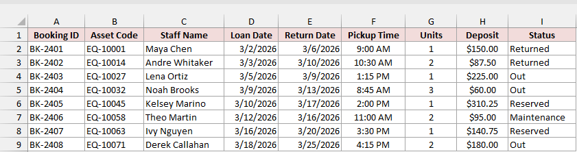
Here are the steps:

1. Select C2:C9 and open Data > Data Validation.

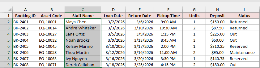
2. Set Allow to Text length and Data to less than or equal to. Enter 30 as the Maximum, then click OK.

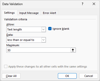
A name with 30 characters is still accepted. Type 31 characters and Excel blocks it.

Use a Custom Formula in Data Validation

When none of the built-in rules fit, set Allow to Custom and give Excel a formula.

Excel accepts the entry when the formula returns TRUE and rejects it when it returns FALSE.

Write the formula for the first cell in your selection. Excel adjusts the relative references for every other cell, just like when you copy a formula down a column.

Method #7: Using COUNTIF to Block Duplicate Entries

No built-in rule can catch a duplicate ID, but a COUNTIF formula can.

Below I have the Loan Register with Booking IDs in A2:A9. Every Booking ID has to be unique.

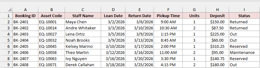
Here are the steps:

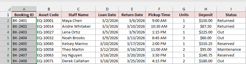
1. Select A2:A9 so that A2 is the active cell, then open Data > Data Validation.

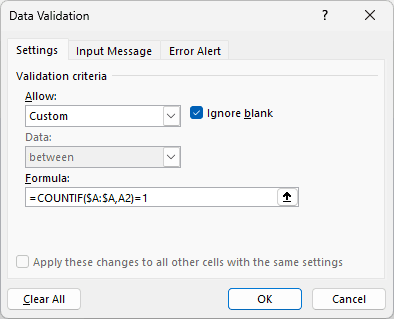
2. Set Allow to Custom and enter the formula below in the Formula box, then click OK.

=COUNTIF($A:$A,A2)=1

Now type BK-2401 into A9. That ID is already in A2, so Excel rejects it.

How does this formula work?

COUNTIF counts how many times the entry in A2 appears in column A. For a unique ID, that count is exactly 1, so the formula returns TRUE.

The column reference $A:$A is absolute, so every cell checks the whole column. A2 is relative, so A3 checks itself, A4 checks itself, and so on.

Note: Because the formula looks at the entire column, you can later apply this rule to more rows (say A2:A500) without changing the formula.

Method #8: Using AND and EXACT to Check a Code Pattern

You can combine several tests in one rule with AND. The entry is accepted only when every test returns TRUE.

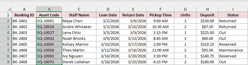
Below I have the Loan Register with Asset Codes in B2:B9. Each code must be a capital EQ- followed by exactly five digits, like EQ-10001.

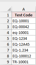
Before applying a formula like this, I like to test it in a helper column. On a Rule Tester sheet, I typed some good and bad codes into A2:A9.

Here is the same test formula, pointed at A2 and filled down to A9:

=AND(EXACT(LEFT(A2,3),"EQ-"),LEN(A2)=8,ISNUMBER(--RIGHT(A2,5)),RIGHT(A2,5)=TEXT(RIGHT(A2,5),"00000"))

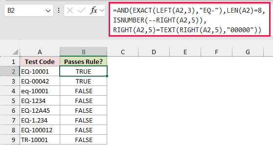
AND collapses its tests into one TRUE or FALSE, so this formula can’t spill. Fill it down instead.

Only EQ-10001 and EQ-00042 return TRUE. The lowercase code, the short one, the one with a letter, the one with a decimal point, and the TR- code all return FALSE.

Once the tests look right, here are the steps to apply the rule:

1. Select B2:B9 so that B2 is the active cell, then open Data > Data Validation.

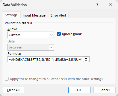
2. Set Allow to Custom and enter the formula below in the Formula box, then click OK.

=AND(EXACT(LEFT(B2,3),"EQ-"),LEN(B2)=8,ISNUMBER(--RIGHT(B2,5)),RIGHT(B2,5)=TEXT(RIGHT(B2,5),"00000"))

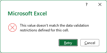
Now try typing eq-10071 into B9. Excel rejects it because the prefix isn’t in capitals.

How does this formula work?

EXACT(LEFT(B2,3),”EQ-“) checks the first three characters. EXACT is case-sensitive, so “eq-” fails. A plain LEFT(B2,3)=”EQ-” would have let it through.

LEN(B2)=8 makes sure the code is exactly eight characters long: three for the prefix and five for the number.

ISNUMBER(–RIGHT(B2,5)) takes the last five characters and checks they can be read as a number. That catches codes like EQ-12A45.

The last test compares those five characters with TEXT(RIGHT(B2,5),”00000″). They only match when all five are digits, so entries like EQ-1.234 fail.

Note: In Microsoft 365, the REGEXTEST function can do the same check in a shorter formula: =REGEXTEST(B2,”^EQ-\d{5}$”). It’s only available in Microsoft 365.

Method #9: Using WEEKDAY to Allow Only Weekdays

The Date rule can’t skip weekends, but a custom formula with WEEKDAY can.

This is useful for due dates, delivery dates, and anything that has to land on a working day.

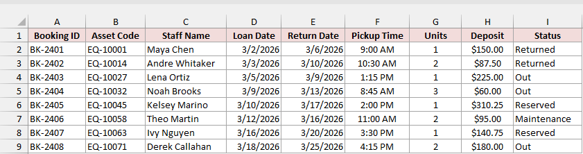
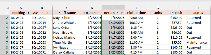
Below I have the Loan Register with Return Dates in E2:E9. The return desk is closed on weekends, so every return date has to be a Monday to Friday.

Here are the steps:

1. Select E2:E9 so that E2 is the active cell, then open Data > Data Validation.

2. Set Allow to Custom and enter the formula below in the Formula box, then click OK.

=WEEKDAY(E2,2)<6

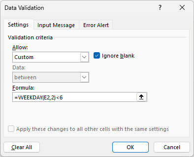
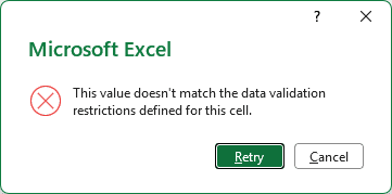
Now try typing 3/28/2026 (a Saturday) into E9. Excel rejects it.

How does this formula work?

With 2 as the second argument, WEEKDAY numbers the days from Monday (1) to Sunday (7).

Monday to Friday return 1 to 5, so the test <6 is TRUE only on weekdays.

Custom Formula Cheat Sheet

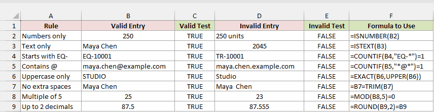
Here are eight more custom rules you can copy. Each formula is written for B2, so change B2 to the first cell of your own selection.

Rule	Formula	Accepts	Rejects
Numbers only	=ISNUMBER(B2)	250	250 units
Text only	=ISTEXT(B2)	Maya Chen	2045
Starts with EQ-	=COUNTIF(B2,"EQ-*")=1	EQ-10001	TR-10001
Contains @	=COUNTIF(B2,"*@*")=1	maya.chen@example.com	maya.chen.example.com
Uppercase only	=EXACT(B2,UPPER(B2))	STUDIO	Studio
No extra spaces	=B2=TRIM(B2)	Maya Chen	Maya Chen (with a double space)
Multiple of 5	=MOD(B2,5)=0	25	23
Up to 2 decimals	=ROUND(B2,2)=B2	87.5	87.555

The COUNTIF wildcard rules aren’t case-sensitive, so “eq-10001” would pass the Starts with EQ- rule. Use EXACT, like in Method #8, when case matters.

The Custom Rules sheet in the example file has all eight rules applied, with a TRUE/FALSE test for a valid and an invalid entry next to each one.

Add an Input Message and Error Alert

A rule works better when people know about it. Here’s how to show a hint before someone types and control the message they see after a bad entry.

Method #10: Adding an Input Message

An input message is a small note that pops up when someone selects a validated cell.

It tells people the rule before they type, so fewer entries get rejected.

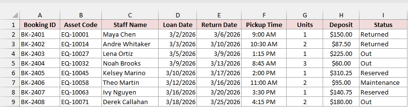
Below I have the Loan Register with the Units column in G2:G9, which only accepts 1 to 5 units.

I want a reminder to show up whenever someone selects one of these cells.

Here are the steps:

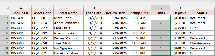
1. Select G2:G9 and open Data > Data Validation.

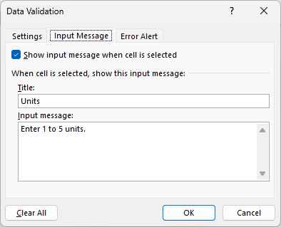
2. Go to the Input Message tab, keep Show input message when cell is selected checked, enter Units as the Title and Enter 1 to 5 units. as the Input message, then click OK.

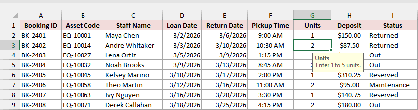
Now when you select any cell in G2:G9, the note shows up next to it.

Method #11: Choosing an Error Alert Style

The Error Alert tab controls what happens when someone types an invalid value. You can write your own title and message, and pick one of three styles:

• Stop: blocks the entry. The person can only retry or cancel.
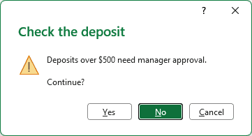
• Warning: asks “Continue?”. Yes keeps the invalid entry, No goes back to editing, and Cancel removes it.
• Information: shows your message. OK keeps the entry and Cancel removes it.

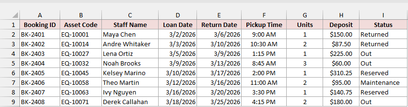
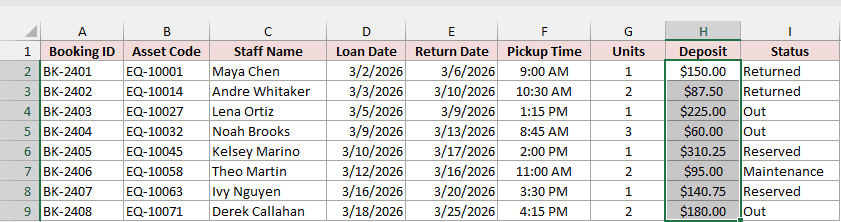
Below I have the Loan Register with Deposits in H2:H9, set to 0 to 500 with the Decimal rule.

A bigger deposit is allowed with a manager’s approval, so I want a warning instead of a hard block.

Here are the steps:

1. Select H2:H9 and open Data > Data Validation.

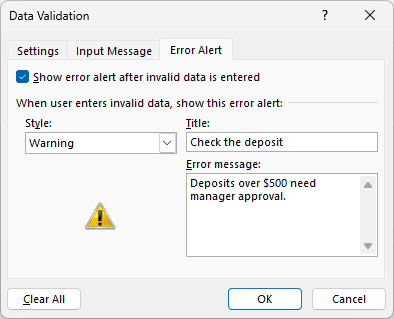
2. Go to the Error Alert tab and set Style to Warning. Enter Check the deposit as the Title and Deposits over $500 need manager approval. as the Error message, then click OK.

Now type 650 into H3. Excel shows your warning, and clicking Yes keeps the value.

Note: Warning and Information alerts let invalid values into the sheet. Use Stop when a wrong value would break something, like a duplicate ID.

Edit, Copy, Find, and Remove Data Validation Rules

Once your rules are in place, you’ll need to change, copy, find, or clear them at some point. Here’s how to do each.

Method #12: Editing an Existing Rule

To change a rule, you reopen the same dialog on a validated cell.

You also want the change to reach every cell that uses the rule, not only the one you selected.

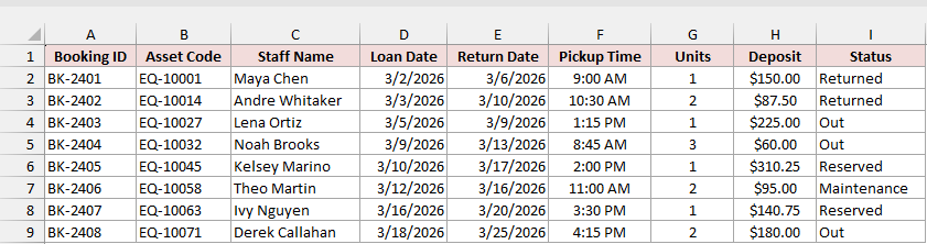
Below I have the Loan Register with all its rules in place. Units in G2:G9 currently accepts 1 to 5, and I want to raise the limit to 10.

Here are the steps:

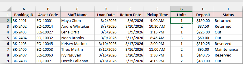
1. Select any one cell in the Units column, like G2, and open Data > Data Validation.

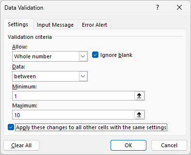
2. Change the Maximum to 10, check Apply these changes to all other cells with the same settings, then click OK.

Excel updates every cell in G2:G9, even though you only selected one.

Method #13: Copying a Rule With Paste Special

When you add new rows to a list, they don’t pick up the rules above them on their own.

Paste Special can copy just the validation rules, without touching the values.

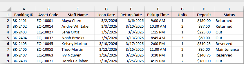
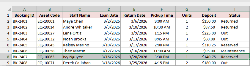
Below I have the Loan Register where rows 2 to 8 have all the rules, but the last booking in row 9 was added later and has none.

Here are the steps:

1. Select A8:I8 (a row that has the rules) and press Ctrl + C.

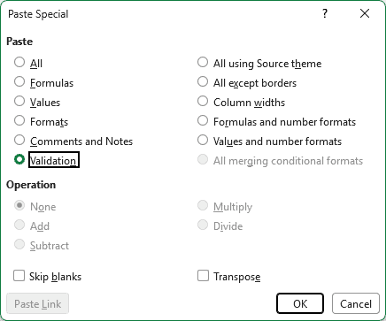
2. Select A9:I9, press Ctrl + Alt + V to open Paste Special, choose Validation, and click OK.

Row 9 now has the same nine rules, and its values stay exactly as they were.

Method #14: Finding Validated Cells With Go To Special

In a workbook someone else built, it’s hard to tell which cells have rules. Go To Special can select all of them at once.

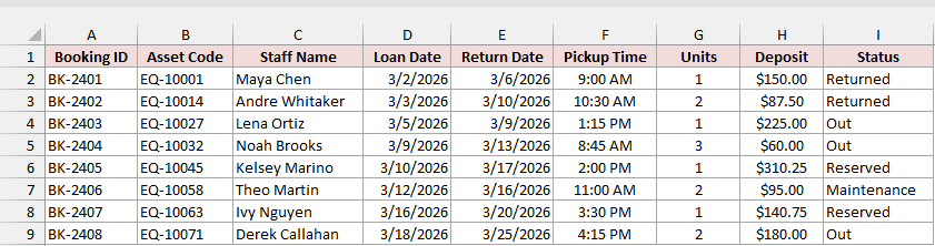
Below I have the Loan Register with rules applied, but nothing on the sheet shows which cells carry one.

Here are the steps:

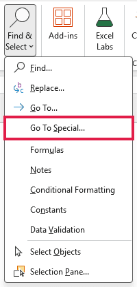
1. On the Home tab, click Find & Select, then Go To Special.

2. Select Data validation, keep All selected, and click OK.

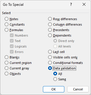
Excel selects every cell with a rule, which here is A2:I9. Choose Same instead of All to find only the cells that share the active cell’s rule.

The Find & Select menu also has a Data Validation item that skips the dialog and selects every validated cell straight away.

Method #15: Using Circle Invalid Data

Data validation only checks values as they’re typed. Values that were already in the cells, or that got pasted in, can still break the rules. Circle Invalid Data finds them.

Below I have the Loan Register with rules applied. Two entries break them: 8 units for BK-2404 and a Saturday return date (3/21/2026) for BK-2406.

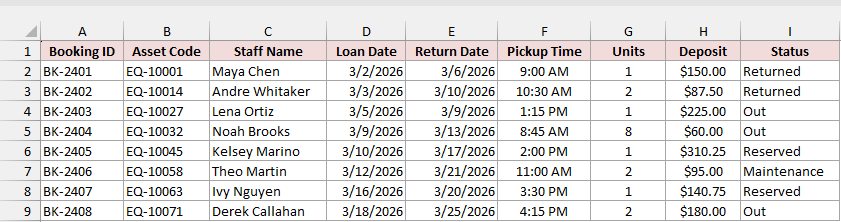
Here are the steps:

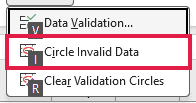
1. On the Data tab, click the arrow next to Data Validation and choose Circle Invalid Data.

Excel draws a red circle around G5 and E7.

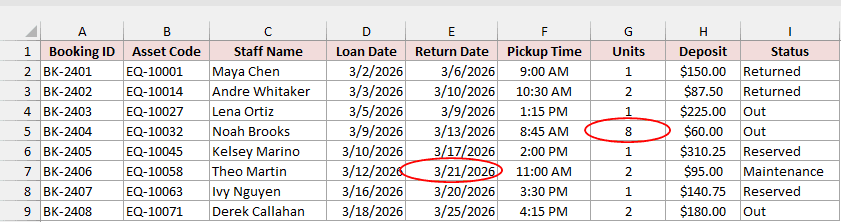
Fix the values and the circles disappear. To remove them without fixing anything, choose Clear Validation Circles from the same menu.

Method #16: Removing Rules With Clear All

Clear All removes data validation from the selected cells and leaves their values in place. It’s how you take off restrictions you no longer need.

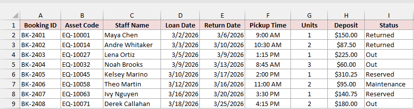
Below I have the Loan Register with rules on A2:I9, and I want to remove all of them.

Here are the steps:

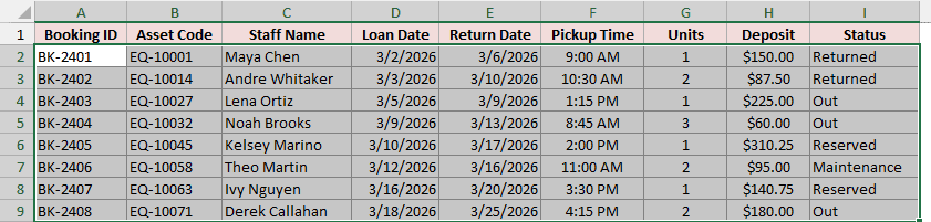
1. Select A2:I9 and open Data > Data Validation. If Excel says the selection contains more than one type of validation, click OK.

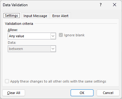
2. Click Clear All, then OK.

To clear the whole sheet, press Ctrl + A first and follow the same steps.

Removing a drop-down works the same way, and there are a few more options in this guide on how to remove a drop-down list in Excel.

Additional Notes About Data Validation in Excel

• Pasting replaces the rule. A normal paste copies the source cell’s validation (or lack of it) over your rule. Use Paste Special > Values to paste data and keep the rule. This is a common reason a drop-down list stops working.
• Only typed entries are checked. Values already in the cells and results of formulas aren’t checked. Use Circle Invalid Data (Method #15) to catch them.
• Protect the sheet to keep the rules. Anyone can open the dialog and click Clear All. Unlock the input cells in Format Cells, then use Review > Protect Sheet.
• A list source can sit on another sheet. Since Excel 2010, the Source box accepts a reference like =’Status Choices’!$A$2:$A$5. A named range still works but isn’t required.
• The example file has every rule applied. Select any cell in the Loan Register and open Data > Data Validation to see its rule, or try typing a bad value.

Frequently Asked Questions

Here are answers to a few common questions about data validation in Excel.

Where is data validation in Excel?

It’s on the Data tab, in the Data Tools group. You can also press Alt, A, V, V.

If the button is grayed out, you may still be editing a cell (press Enter or Esc). It’s also unavailable on a protected sheet or in a shared workbook.

Can data validation make a cell required?

No. Validation only runs when someone types into a cell, so a cell nobody touches stays blank, whether or not Ignore blank is checked.

To spot missing entries, use a check like =COUNTBLANK(C2:C9), which returns the number of empty cells, or highlight blanks with conditional formatting.

Can I apply two data validation rules to the same cell?

No, each cell holds one rule. To check two conditions, combine them in a Custom formula with AND (both must pass) or OR (either can pass), like in Method #8.

How do I make a data validation drop-down list update automatically?

In Excel 2021 or later, put a formula like =SORT(UNIQUE(A2:A50)) next to your item list, say in K2. Then enter =$K$2# as the list’s Source.

The # tells Excel to use the whole spill range, so the drop-down grows and shrinks as the formula’s results change.

Conclusion

In this article, I showed you how to add drop-down lists, number, date, time, and text length rules, and custom formula rules in Excel.

I also covered input messages, error alerts, and how to edit, copy, find, and remove rules.

For most fields, a built-in rule like List or Whole number is enough. When it isn’t, a custom formula can check things like duplicate IDs or exact code patterns.

I hope you found this article helpful.

Other Excel articles you may also like:

• Using Less Than or Equal to Operator in Excel Formula
• How to Group Duplicates in Excel
• How to Select Multiple Items from a Drop Down in Excel?
• Create a Drop-down List with Color in Excel