How to Use Slicers in Excel (Beginner to Advanced Guide)

Slicers in Excel turn a PivotTable or Table filter into a set of buttons. Click East, and the report shows East. Click West, and it switches.

That’s easier than opening a filter drop-down and ticking boxes. It’s also easier to read, because the highlighted buttons tell anyone looking at the sheet exactly what’s filtered.

Once one slicer works, you can go further. Two slicers can filter together, one slicer can drive a chart or two PivotTables, and a Timeline filters dates.

In this article, I’ll show you how to add a slicer to a PivotTable or Table, filter with several buttons, add a Timeline, and format your slicers.

How to Insert a Slicer in a PivotTable

A PivotTable is the most common place to use a slicer. The slicer sits next to the report, and every click changes the numbers the PivotTable shows.

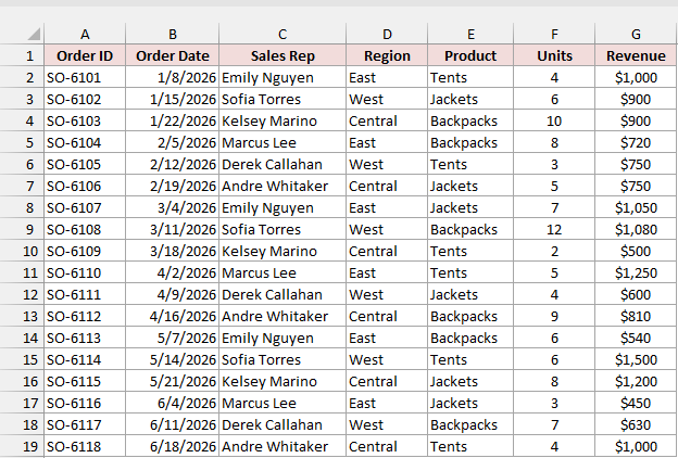
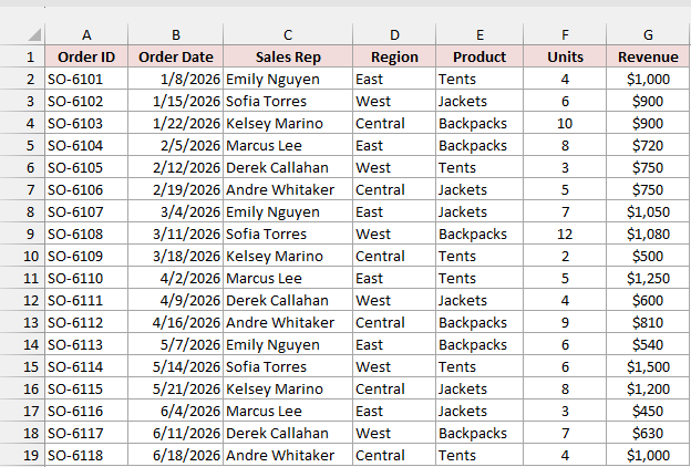
Below I have a dataset of 18 sales orders for an outdoor gear store.

Each order has a date, a sales rep, a region, a product, the units sold, and the revenue.

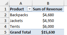
I’ve made a PivotTable from this data that shows the total revenue for each product. The grand total is $15,630.

Now I want to filter this PivotTable by region with a slicer.

Here are the steps to insert a slicer in a PivotTable:

1. Select any cell in the PivotTable.
2. Go to the PivotTable Analyze tab and click Insert Slicer.

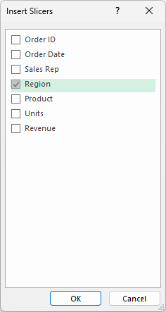
3. In the Insert Slicers dialog box, check Region and click OK.

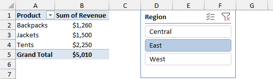
Excel adds a Region slicer with one button for each region in the data: Central, East, and West.

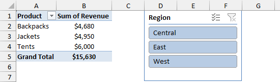
All three buttons are highlighted, which means nothing is filtered yet. Click East, and the PivotTable now shows only the East orders. The grand total drops to $5,010.

NOTE: Slicers for PivotTables work in Excel 2010 and later versions. You can also go to Insert and click Slicer with a cell in the PivotTable selected.

How to Add a Slicer to an Excel Table (No PivotTable Needed)

You don’t need a PivotTable to use a slicer. An Excel Table can have one too, and it filters the rows of the Table directly.

Below I have the same 18 sales orders. It’s a normal range right now, so I’ll turn it into a Table first.

Here are the steps to add a slicer to an Excel Table:

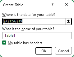
1. Select any cell in the data and press Ctrl + T. Make sure My table has headers is checked, then click OK.

2. Go to the Table Design tab and check Total Row, then click Insert Slicer.
3. Check Region and click OK.

Now click West in the slicer. The Table hides every order that isn’t from the West region, and only six rows are left.

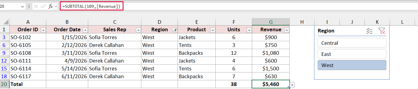
Look at the Total Row. It shows $5,460, which is the revenue for the six visible rows only. That’s because the Total Row uses this formula:

=SUBTOTAL(109,[Revenue])

SUBTOTAL with 109 adds only the visible rows, so it changes every time you click a slicer button.

A regular SUM formula would keep showing $15,630, because it adds the hidden rows too.

NOTE: Slicers for Excel Tables need Excel 2013 or later. A Table slicer filters the Table’s rows, while a PivotTable slicer filters the PivotTable’s summary. Neither one changes the other.

Filtering With Slicer Buttons (Select, Multi-Select, and Clear)

Once a slicer is in place, all the filtering happens with clicks. Here I’m back to the revenue PivotTable with its Region slicer, where all three regions are showing.

To show one item, click its button. Excel removes every other item from the filter.

To show more than one item, you have three options:

• Hold Ctrl and click each button you want.
• Click the Multi-Select button in the slicer’s header. Each click then adds or removes a button without clearing the others.
• Select the slicer and press Alt + S to turn Multi-Select on or off.

Here I’ve selected East and West together. The PivotTable adds up both regions, so the grand total is $10,470.

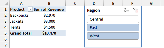
To remove the filter, click the Clear Filter button in the slicer’s top-right corner, or select the slicer and press Alt + C.

All the buttons light up again, and the PivotTable goes back to $15,630.

Using Two Slicers Together

You can add more than one slicer to the same PivotTable. The slicers work together, so a click in one slicer changes what’s available in the other.

Here I’ve added a Sales Rep slicer next to the Region slicer, and I’ve clicked East.

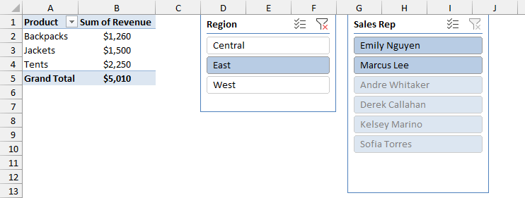
Only Emily Nguyen and Marcus Lee are still dark in the Sales Rep slicer.

The other four reps are faded and moved to the bottom, because none of them sold anything in the East region.

That’s a slicer’s way of telling you which buttons will return data. You can still click a faded button, but the PivotTable will be empty.

Now I’ll click Emily Nguyen in the Sales Rep slicer. The PivotTable shows only Emily’s East orders, for a total of $2,590.

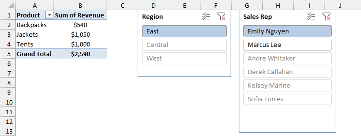
The Region slicer changes too. Central and West are now faded, because Emily only sells in the East.

Using a Slicer With a PivotChart

A PivotChart is a chart built on a PivotTable, so any slicer connected to that PivotTable filters the chart as well.

Here are the steps to add a PivotChart that the slicer controls:

1. Select any cell in the revenue PivotTable that already has a Region slicer.
2. Go to the PivotTable Analyze tab, click PivotChart, pick Clustered Column, and click OK.

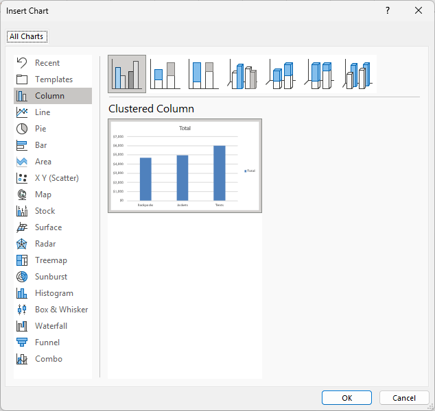
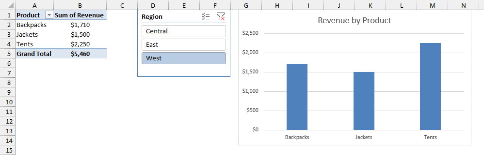
Now click West in the Region slicer. The PivotTable and the chart both switch to West, with Tents on top at $2,250.

Filtering Dates With a Timeline

A Timeline is a slicer made for dates. Instead of one button per date, it shows a bar of months that you drag across to pick a period.

Here I’m starting again from the revenue PivotTable with no slicers. The data has an Order Date column that runs from January to June 2026.

Here are the steps to add a Timeline:

1. Select any cell in the PivotTable.
2. Go to the PivotTable Analyze tab and click Insert Timeline.

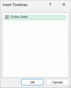
3. In the Insert Timelines dialog box, check Order Date and click OK.

Drag across January, February, and March in the Timeline. The label changes to Q1 2026, and the PivotTable shows only first-quarter revenue, which is $7,650.

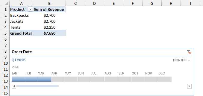
Click the MONTHS drop-down on the right of the Timeline to switch to years, quarters, or days.

NOTE: Timelines work only with PivotTables, not with Excel Tables, and need Excel 2013 or later. The date column must hold real dates, not text that looks like dates.

Connecting One Slicer to Multiple PivotTables

One slicer can filter more than one PivotTable at the same time. This works when the PivotTables are built from the same data source.

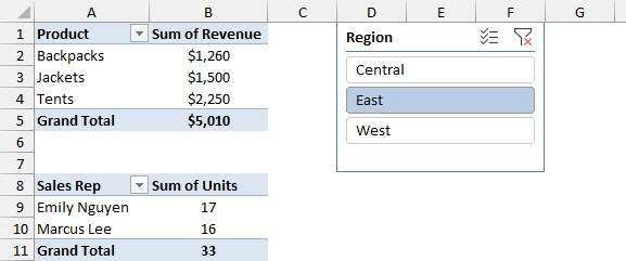
Here I have two PivotTables from the same sales data: revenue by product, and units by sales rep. The Region slicer is connected to the first one only.

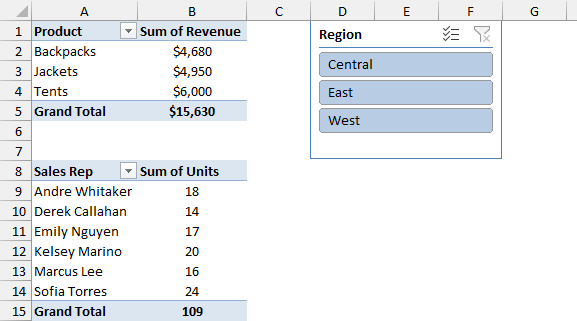
Here are the steps to connect the slicer to the second PivotTable:

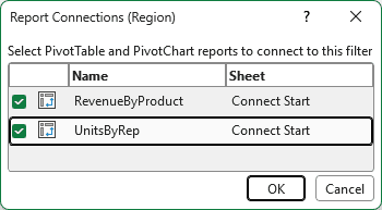
1. Select the slicer, go to the Slicer tab, and click Report Connections.
2. Check the PivotTable you want the slicer to control and click OK.

Now click East in the slicer. Both PivotTables filter together, and the units PivotTable shows only Emily Nguyen and Marcus Lee.

If the PivotTable you want isn’t in the Report Connections list, it’s built on a different data source.

I cover that case in my guide on how to connect a slicer to multiple pivot tables.

Changing Slicer Style, Columns, and Size

A new slicer is a tall, narrow box with blue buttons.

You can change its colors, lay the buttons out side by side, and resize it from the Slicer tab, which appears when you select the slicer.

These are the main options on the Slicer tab:

• Slicer Styles: pick a new color scheme for the slicer from the gallery.
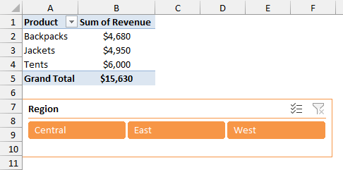
• Columns: set how many columns of buttons the slicer shows. Set it to 3 for a region slicer, and the buttons sit in one row.
• Height and Width in the Buttons group: change the size of each button.
• Height and Width in the Size group: change the size of the whole slicer.

Here I’ve picked an orange style from the Dark section, set Columns to 3, and made the slicer wide and short. It now fits neatly under the PivotTable.

Changing Slicer Settings

Some slicer options aren’t on the ribbon. They’re in the Slicer Settings dialog box, which you open by right-clicking the slicer and choosing Slicer Settings.

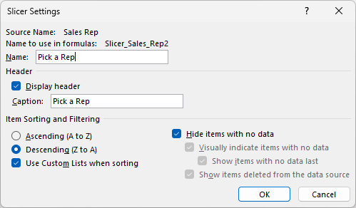
These are the settings you’ll use most:

• Caption: the title that shows at the top of the slicer.
• Display header: uncheck it to hide the title bar, along with the Multi-Select and Clear Filter buttons.
• Sorting: show the items in ascending or descending order.
• Hide items with no data: remove buttons that would return nothing, instead of fading them.

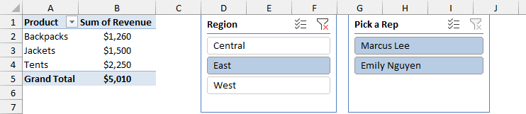
Here I’ve changed the Sales Rep slicer’s caption to “Pick a Rep”, sorted it Z to A, and turned on Hide items with no data.

When I click East in the Region slicer, the rep slicer shows only Marcus Lee and Emily Nguyen. The four reps with no East sales disappear instead of fading.

Locking a Slicer and Protecting the Sheet

A slicer moves when you insert or resize columns next to it. If you’ve laid out a report carefully, you’ll want it to stay put.

Here are the steps to stop a slicer from moving and let people use it on a protected sheet:

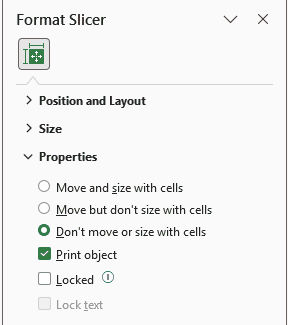
1. Right-click the slicer and choose Size and Properties.
2. Under Properties, pick Don’t move or size with cells, and uncheck Locked.

3. Go to the Review tab and click Protect Sheet. Check Use PivotTable and PivotChart (or Use AutoFilter for a Table slicer), then click OK.

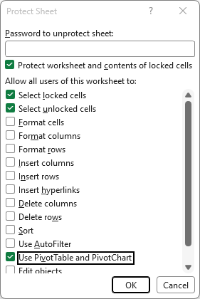
The sheet is now protected, so nobody can type over the PivotTable, but the slicer buttons still work.

Disconnecting or Deleting a Slicer

To stop a slicer from filtering a PivotTable without deleting it, select the slicer, go to Slicer > Report Connections, and uncheck that PivotTable.

To delete a slicer, click its border to select it and press Delete. You can also right-click it and choose Remove “Region”, where “Region” is the slicer’s name.

Deleting a slicer doesn’t remove the filter it applied. Clear the filter first (Alt + C), or the PivotTable or Table stays filtered after the slicer is gone.

Slicers vs Filters in Excel

Slicers and the regular filter drop-downs do the same basic job. The difference is in how easy they are to use and read.

	Slicer	Filter drop-down
How you filter	Click a button	Open a list and tick boxes
Shows what’s filtered	Yes, highlighted buttons	Only a small funnel icon
Works on	PivotTables and Tables	Any range, Table, or PivotTable
Filters several PivotTables	Yes, with Report Connections	No
Takes up space on the sheet	Yes	No
Filter by condition (greater than, contains)	No	Yes

Use a slicer when other people will filter the report, or when you want the filter to be visible.

Stick with the drop-down when you need a condition, such as orders above $1,000.

Why Insert Slicer Is Greyed Out (and Other Slicer Problems)

Insert Slicer is greyed out. Check these, in order:

• The active cell is inside the Table or PivotTable. Excel only enables the button when one of them is selected.
• The workbook isn’t in Compatibility Mode. An .xls file can’t have slicers, so save it as .xlsx.
• The PivotTable wasn’t made in a very old version of Excel. Slicers only work with PivotTables created in Excel 2007 or later, so rebuild an old one.
• Objects aren’t hidden. If Ctrl + 6 was pressed by accident, press it again to show objects.

A PivotTable is missing from Report Connections. The PivotTable uses a different data source, so the slicer can’t reach it. Rebuild it from the same source.

The slicer still shows items that are gone from the data. Right-click the PivotTable and choose PivotTable Options.

On the Data tab, set Number of items to retain per field to None, then refresh the PivotTable.

You can also uncheck Show items deleted from the data source in the slicer’s Slicer Settings.

Additional Notes About Slicers in Excel

• A PivotTable slicer shows the items in the PivotTable’s cache, so new regions or products appear only after you refresh the PivotTable.
• Build your PivotTable from an Excel Table. New rows added to the Table flow into the PivotTable on refresh, so your slicer never misses data.
• In the example file, the Sales Dashboard sheet has both PivotTables, the two slicers, the Timeline, and the chart already connected, so you can click around right away.

Frequently Asked Questions

Can I use a slicer without a PivotTable?

Yes. Convert your data to an Excel Table with Ctrl + T, then go to Table Design > Insert Slicer. This needs Excel 2013 or later.

Why doesn’t my SUM formula change when I click a slicer?

SUM adds every row, including the ones a slicer hides. Use SUBTOTAL with 109 instead, or turn on the Table’s Total Row, which uses SUBTOTAL for you.

Do slicers work on a Mac and in Excel for the web?

On a Mac, slicers work in Excel 2016 and later, and you Cmd-click to pick several items.

In Excel for the web, you can use any slicer and insert new ones for PivotTables. Slicers for Tables need the desktop app.

Can I search inside a slicer?

No, slicers don’t have a search box. For a long list, set Columns to 2 or 3, or turn on Hide items with no data.

Can a slicer sit on a different sheet from its PivotTable?

Yes. Select the slicer, press Ctrl + X, go to the other sheet, and press Ctrl + V. It stays connected, which is handy for a dashboard sheet.

Conclusion

I showed you how to insert a slicer in a PivotTable and a Table, filter with several buttons, and add a second slicer, a chart, and a Timeline.

I also covered formatting, settings, locking, and fixes for common problems. I hope you found this article helpful.

Other Excel articles you may also like:

• How to Group by Months in Excel Pivot Table?
• How to Group by Quarters in Excel Pivot Table?
• How to Sort a Pivot Table in Excel?
• How to Lock a Pivot Table in Excel
• How to Clear Pivot Table Cache?