If you want to run quick calculations on a filtered list and have the result update automatically as you change the filter, the SUBTOTAL function in Excel is what you’re after.
It can sum, average, count, find the min, max, and a handful more, all while ignoring rows that are filtered out.
In this article, I’ll walk you through how the SUBTOTAL function works, what the 11 function codes do, the difference between the 1-11 and 101-111 ranges, and a few examples that show why it’s so useful.
SUBTOTAL itself returns a single value, so it doesn’t spill on its own. What makes it useful in a dynamic-array world is composition: you can wrap it around a FILTER result or a spilled range with the # operator, and the filter-awareness still applies.
SUBTOTAL Function Syntax
Here is the syntax of the SUBTOTAL function:
=SUBTOTAL(function_num, ref1, [ref2], ...)
- function_num – A number from 1-11 or 101-111 that tells SUBTOTAL which calculation to run (sum, average, count, etc.)
- ref1 – The first range you want to run the calculation on
- [ref2], … – Optional additional ranges. You can pass up to 254 of them
When to Use SUBTOTAL
Use this function when you need to:
- Calculate totals on a filtered list that should update as the filter changes
- Sum or count only the visible rows after hiding some manually
- Avoid double-counting when you have other SUBTOTAL formulas inside the same range
- Reduce a spilled dynamic array (like the result of a FILTER) to a single visible-only total
Let me show you how this all works.
What the Function Codes Mean
The first argument decides which calculation SUBTOTAL runs. There are 11 calculations to pick from, and each one has two codes you can use.
Here are the codes:
| Calculation | 1-11 (includes manually hidden rows) | 101-111 (ignores manually hidden rows) |
|---|---|---|
| AVERAGE | 1 | 101 |
| COUNT | 2 | 102 |
| COUNTA | 3 | 103 |
| MAX | 4 | 104 |
| MIN | 5 | 105 |
| PRODUCT | 6 | 106 |
| STDEV | 7 | 107 |
| STDEVP | 8 | 108 |
| SUM | 9 | 109 |
| VAR | 10 | 110 |
| VARP | 11 | 111 |
Both ranges always ignore rows that are filtered out. The only difference shows up when you hide rows manually (right-click then Hide).
Codes 1-11 still count those hidden rows. Codes 101-111 skip them.
If your data set does not have manually hidden rows, the two ranges behave the same way and you can use either one.
Example 1: Sum a Filtered List
Let’s start with the example that makes SUBTOTAL famous.
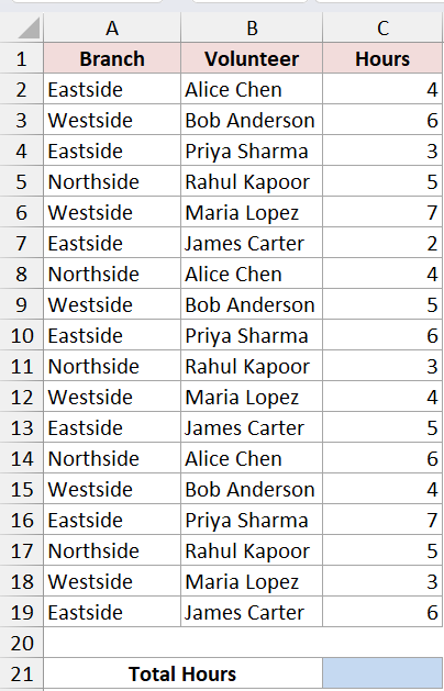
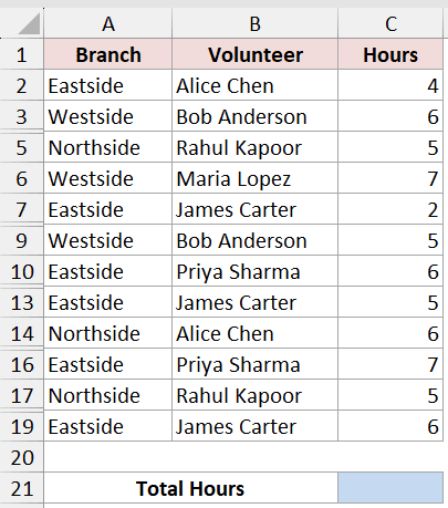
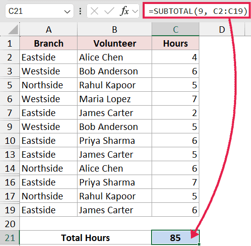
Below is a community library volunteer log. Column A has the branch the volunteer worked at, column B has the volunteer’s name, and column C has the hours they put in that day.
I want a total at the top that updates whenever I filter the list.
Here is the formula:
=SUBTOTAL(9, C2:C19)
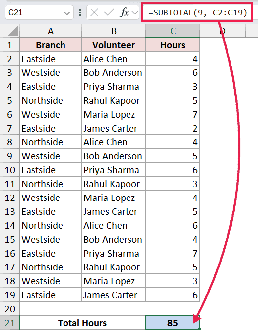
The 9 tells SUBTOTAL to run a SUM on the range C2:C20. Now if you turn on a filter and pick only one branch, the formula recalculates and shows just the hours for that branch.
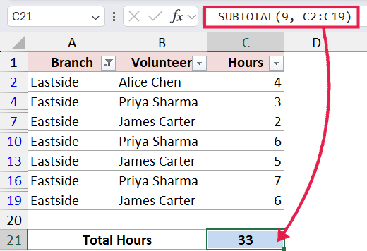
A regular SUM formula would still show the total for the full range, even if half the rows are hidden by the filter.
This is the killer feature of SUBTOTAL. The result follows what you can see on screen.
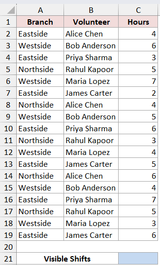
Example 2: Count Visible Rows Only
Here’s another practical scenario.
You filter a list and want a quick count of how many rows are showing.
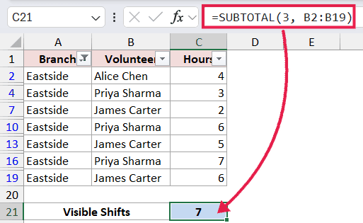
Same volunteer log. I want to count how many shifts are currently visible after the filter is applied.
Here is the formula:
=SUBTOTAL(3, B2:B19)
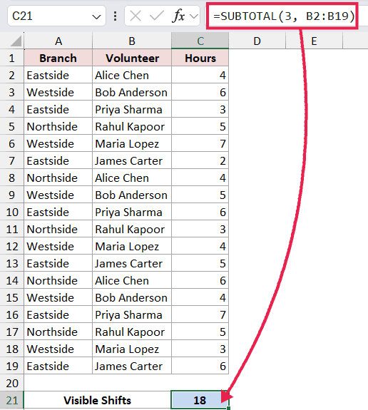
The 3 stands for COUNTA, which counts non-empty cells.
As you filter the list, the count updates to match the visible rows. Drop the filter and the count goes back up.
If you want to count only numbers, use 2 instead of 3 (that’s the COUNT version). For most filtered-list situations, COUNTA (3) is the one you want because it counts text too.
Example 3: Sum When Rows Are Manually Hidden
Now for the case where the 1-11 vs 101-111 difference actually matters.
Same dataset, but instead of using a filter, I right-click on a few rows and pick Hide (maybe to focus on weekend shifts only). I want the total at the top to skip those hidden rows.
Here is the formula:
=SUBTOTAL(109, C2:C19)
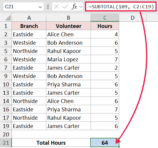
Notice the 109 instead of 9. Both run a SUM, but 109 also ignores any rows you hid manually.
If you used 9 here, the formula would still include the hidden rows in its total.
Quick rule of thumb. If your data is being hidden by a filter, either code works. If your data is being hidden by Hide / Group / Outline, use the 101-111 range.
Example 4: SUBTOTAL Skips Other SUBTOTAL Formulas
This is the gotcha that trips a lot of people up, and it’s actually a feature.
Say you have a long volunteer log with branch headers, and below each branch you’ve got a =SUBTOTAL(9, ...) formula that totals just that branch (highlighted in yellow color). At the very bottom, you want a grand total of the whole log.
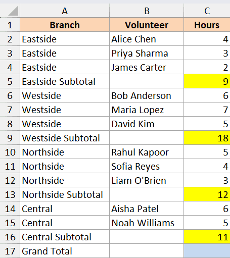
Here is the formula at the bottom:
=SUBTOTAL(9,C2:C16)
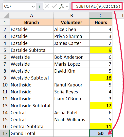
Even though the range C2:C16 includes the per-branch subtotal cells (highlighted in yellow), SUBTOTAL automatically skips any other SUBTOTAL formula inside its range.
So you don’t get double-counted numbers.
A plain SUM in the same spot would add the subtotals on top of the row values and double everything up.
SUBTOTAL vs SUM
Most people reach for SUM by default and only switch to SUBTOTAL when they hit a wall. Here’s the short version of when each one wins.
- SUM is fine when you want a fixed total across the whole range (here’s a full guide on summing a column in Excel), no matter what’s filtered or hidden
- SUBTOTAL is the one to use when you want the total to follow the filter, ignore manually hidden rows, or skip nested subtotals
If you’re building a report that someone will filter, default to SUBTOTAL. It’s what the filtered total row in an Excel Table uses too.
SUBTOTAL vs AGGREGATE
If you’ve come across the AGGREGATE function, it does roughly the same job as SUBTOTAL but with more options.
It can also ignore errors and nested SUBTOTAL/AGGREGATE formulas, supports 19 different calculations instead of 11, and handles array formulas.
Stick with SUBTOTAL for everyday filtered lists and quick visible-row totals. Reach for AGGREGATE when your range has errors you want to skip past, or when you need calculations like LARGE, SMALL, MEDIAN, or PERCENTILE on a filtered range.
SUBTOTAL with code 4 (or 104) also works as a filter-aware way to find the largest value in Excel.
Tips & Common Mistakes
- SUBTOTAL composes with spilled ranges. If a FILTER, UNIQUE, or SORT formula spills into
F2, you can sum its visible result with=SUBTOTAL(9, F2#). The#references the whole spilled output, and SUBTOTAL still respects any filter applied to the rows feeding into it. - You can’t nest SUBTOTAL inside another SUBTOTAL across different ranges to chain calculations. It just skips them. If you need that, use helper columns or AGGREGATE.
- The function_num must be a number, not text.
=SUBTOTAL("9", C2:C20)throws a #VALUE! error. Drop the quotes. - Codes 1-11 and 101-111 act the same when filtering. The 100-series only behaves differently for manually hidden rows. So if you only ever filter, both are fine.
- SUBTOTAL ignores hidden rows but not hidden columns. If you hide column C, SUBTOTAL still uses it. There’s no column equivalent of the 100-series.
- The SUBTOTAL function only works on vertical ranges. If you pass a horizontal range and start hiding columns, it won’t follow you.
- Watch out when copying filtered cells. Filtered SUBTOTAL totals follow the filter, but if you paste the filtered results elsewhere, the formula recalculates against the new range and the number can change.
That covers the main things.
SUBTOTAL is one of those functions that looks plain on paper but earns its keep the moment you start filtering data.
Once you get used to using 9 and 109 instead of plain SUM, and pairing SUBTOTAL with FILTER or a spilled range when you need a slice that doesn’t depend on the AutoFilter UI, you’ll wonder why you didn’t switch sooner.
Related Excel Functions / Articles: