
Getting unique values with criteria in Excel means keeping one copy of each value, but only from rows that meet your conditions.
You might need a customer list for one region or the people confirmed for a particular event. Removing duplicates from the whole column would include people outside that group.
Filter the matching rows first, then extract the unique values from that smaller list.
I’ll show you how to do this with UNIQUE and FILTER, Advanced Filter, and Power Query, including formulas for multiple conditions and blank cells.
Method #1: Using UNIQUE and FILTER
The FILTER function returns values from matching rows. Wrapping it in UNIQUE removes repeated values from that filtered list.
This is the method I’d start with when the list needs to update as your data or criteria change. It works in Microsoft 365, Excel 2021, and Excel 2024.
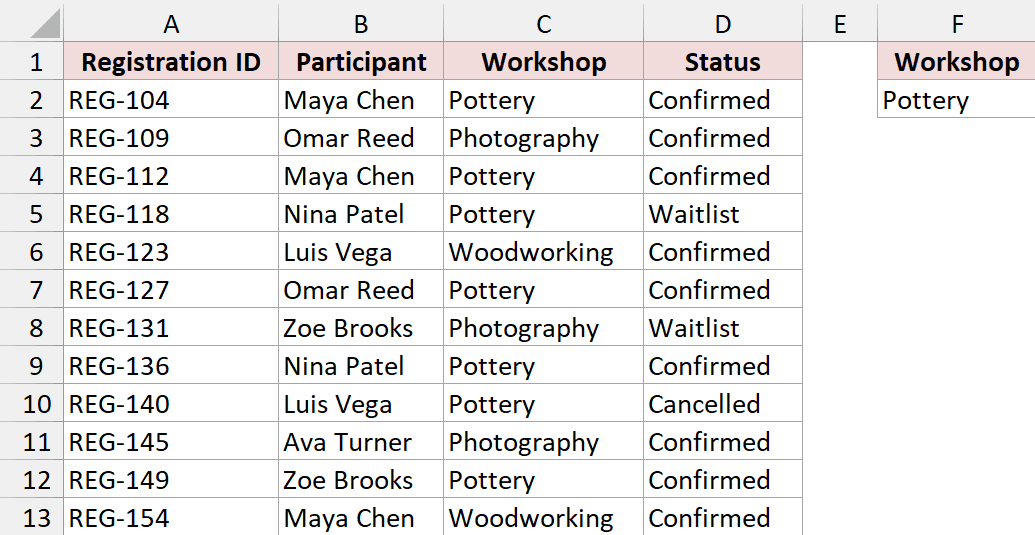
Below I have workshop registrations in A1:D13 on the 1.1 One Condition sheet. Some participants registered more than once, and I want each Pottery participant listed once.
Extract Unique Values With One Condition
Cell F2 contains Pottery. Enter this formula in H2:
=UNIQUE(FILTER(B2:B13,C2:C13=F2))
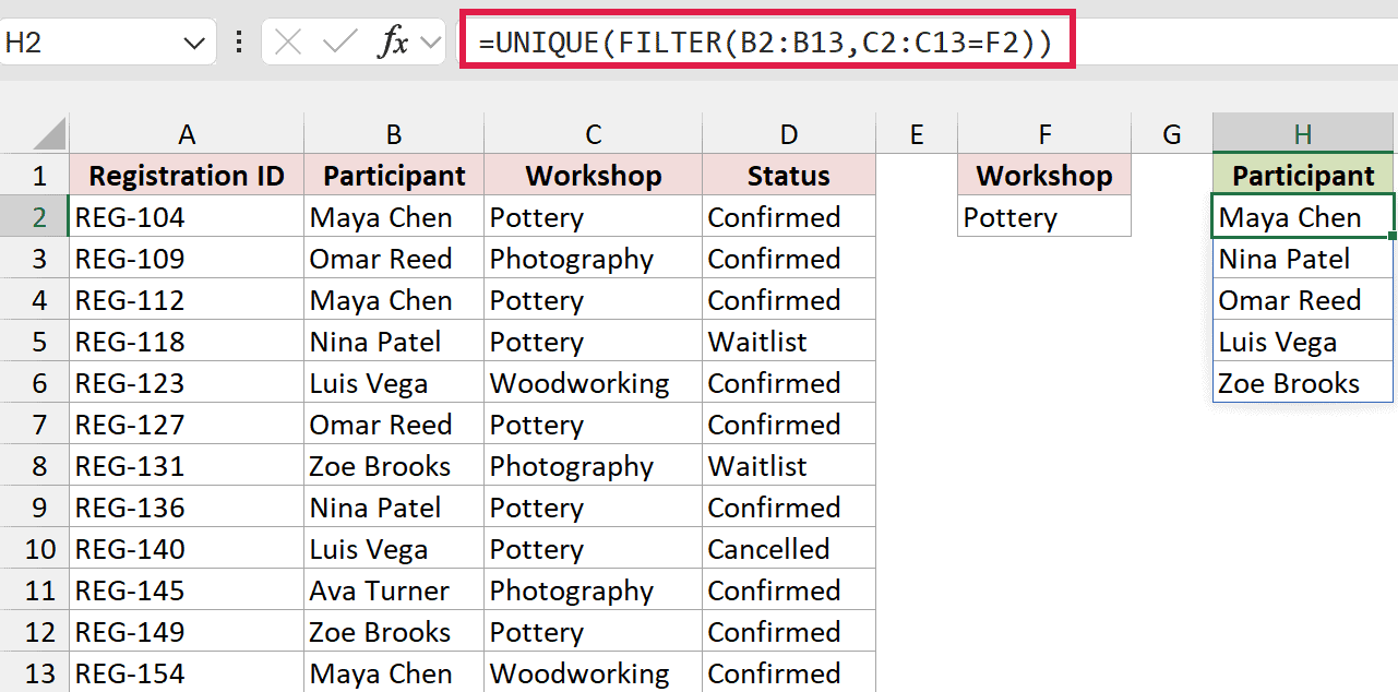
The result is Maya Chen, Nina Patel, Omar Reed, Luis Vega, and Zoe Brooks. Maya appears twice in the Pottery registrations but only once in the result.
How does this formula work?
C2:C13=F2 checks each workshop against Pottery. FILTER returns the corresponding names from B2:B13, and UNIQUE keeps one copy of each name.
The formula spills down the column automatically. Leave the cells below H2 empty so Excel has room for the results.
Extract Unique Values With Multiple AND Conditions
Now I want people whose workshop is Pottery and whose status is Confirmed. Both conditions must be true for the same registration.
On the 1.2 AND Conditions sheet, F2 contains Pottery and F5 contains Confirmed. Enter this formula in H2:
=UNIQUE(FILTER(B2:B13,(C2:C13=F2)*(D2:D13=F5)))
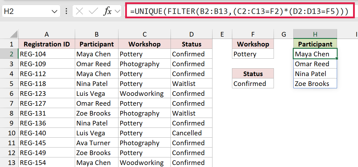
The result is Maya Chen, Omar Reed, Nina Patel, and Zoe Brooks. Luis is excluded because his Pottery registration is Cancelled.
The multiplication sign (*) joins the tests with AND logic. A row passes only when both tests are TRUE.
Nina is included because she has a Confirmed Pottery registration, even though another registration for her is on the waitlist.
Extract Unique Values With OR Conditions
For a list containing participants from Pottery or Photography, a row only needs to match one workshop.
On the 1.3 OR Conditions sheet, F2 contains Pottery and F3 contains Photography. Enter this formula in H2:
=UNIQUE(FILTER(B2:B13,(C2:C13=F2)+(C2:C13=F3)))
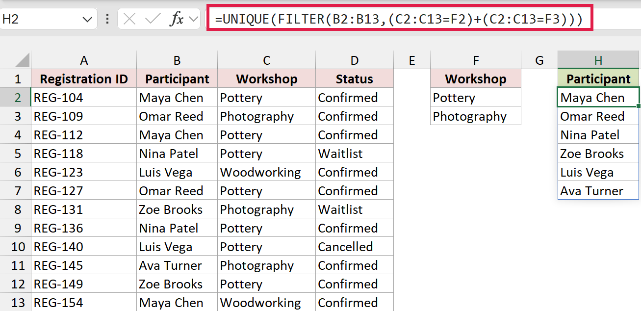
The result is Maya Chen, Omar Reed, Nina Patel, Zoe Brooks, Luis Vega, and Ava Turner.
The plus sign (+) joins the tests with OR logic. FILTER keeps a row when either test is TRUE, and UNIQUE removes repeated names afterward.
This example includes every status. It doesn’t carry over the Confirmed condition from the formula above.
Sort the Unique List Alphabetically
UNIQUE returns names in their first-occurrence order. To alphabetize them, wrap the original formula in the SORT function.
On the 1.4 Sorted List sheet, F2 contains Pottery. Enter this formula in H2:
=SORT(UNIQUE(FILTER(B2:B13,C2:C13=F2)))
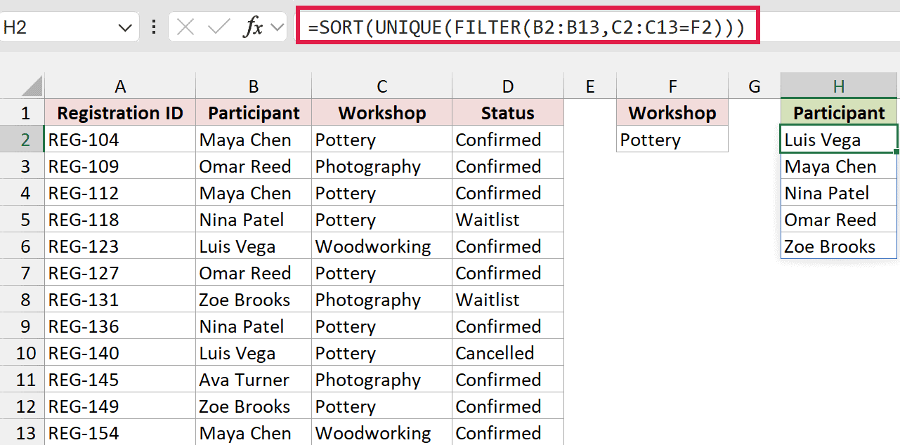
The list now starts with Luis Vega, followed by Maya Chen, Nina Patel, Omar Reed, and Zoe Brooks.
Ignore Blank Names and Handle No Matches
An incomplete registration can leave a blank participant name. On the 1.5 Ignore Blanks sheet, B9 is empty.
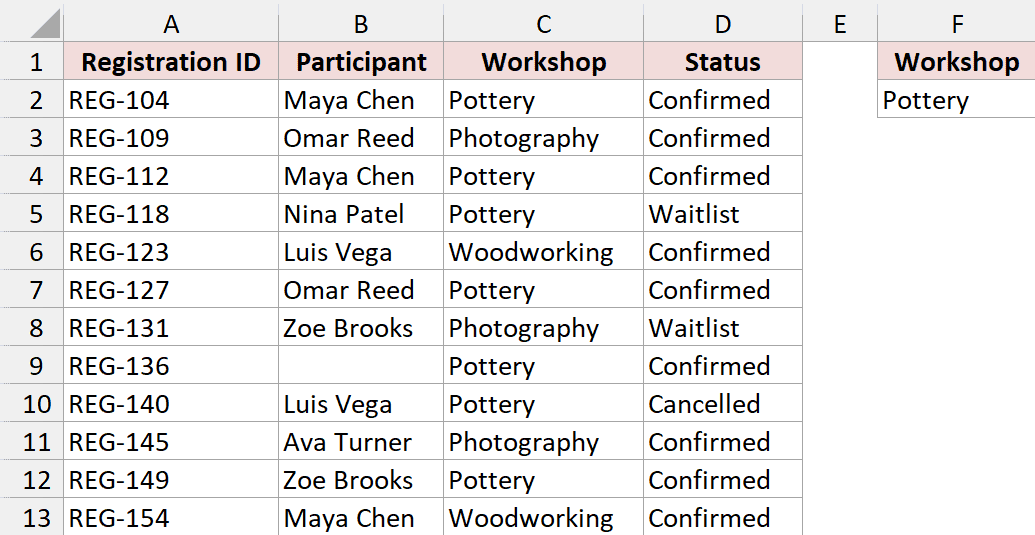
Add a test that requires the participant cell to be nonblank. With Pottery in F2, enter this formula in H2:
=UNIQUE(FILTER(B2:B13,(C2:C13=F2)*(B2:B13<>""),"No matches"))
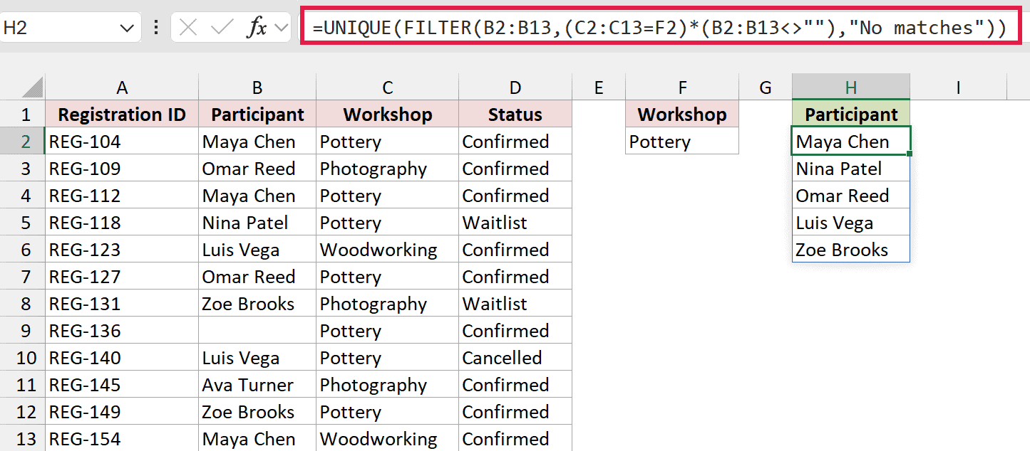
B2:B13<>"" excludes empty cells and formulas returning empty text. Nina still appears because her other Pottery registration has a name.
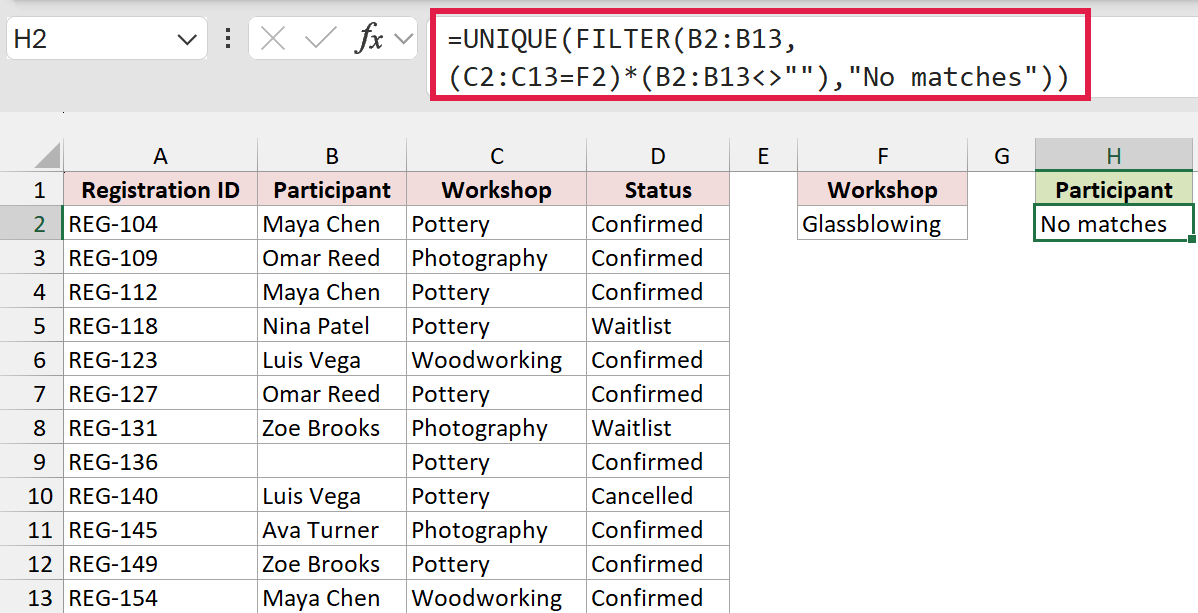
The final FILTER argument, "No matches", supplies a message when no rows qualify. Without that argument, an empty result returns a #CALC! error.
You can see this on the 1.6 No Matches sheet. F2 contains Glassblowing, which isn’t in the registration data. H2 uses this formula:
=UNIQUE(FILTER(B2:B13,(C2:C13=F2)*(B2:B13<>""),"No matches"))
Note: Put the spill formula outside an Excel Table. The source data can be a Table, but the cells receiving the spilled results must be in the ordinary worksheet grid.
Method #2: Using Advanced Filter
Advanced Filter can copy a distinct list to another location without a formula. It’s useful for a one-time extract, including in Excel versions without UNIQUE.
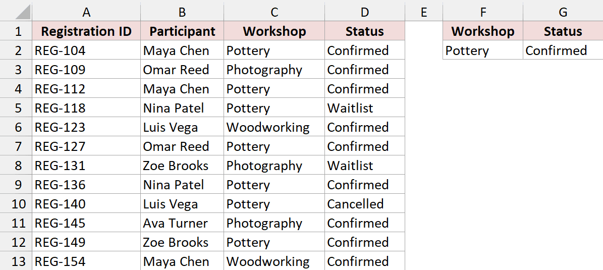
On the 2 Advanced Filter sheet, the registrations occupy A1:D13. I want each participant with a Confirmed Pottery registration listed once in column I.
Here are the steps in desktop Excel for Windows:
- Set up the criteria in F1:G2: Workshop and Status above Pottery and Confirmed. Type Participant in I1 as the output header.
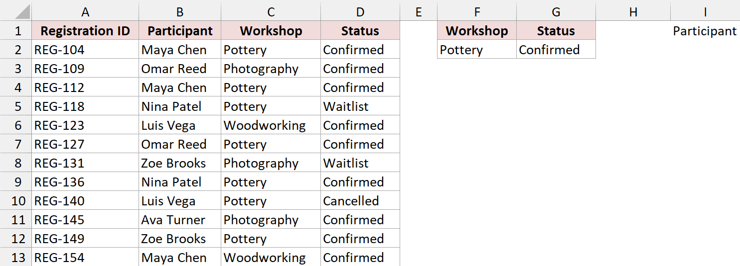
The criteria headers must match the source headers. Conditions on the same row mean AND, so this extract requires both Pottery and Confirmed.
Plain-text Advanced Filter criteria match the beginning of a cell. Pottery works for these categories, but would also match Pottery Basics if that appeared in your data.
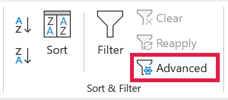
- Select a cell in A1:D13. On the Data tab, click Advanced in the Sort & Filter group.
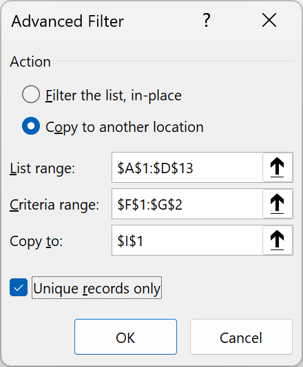
- Choose Copy to another location. Set List range to $A$1:$D$13, Criteria range to $F$1:$G$2, and Copy to to $I$1. Check Unique records only.
- Click OK to copy the matching participant names into column I.
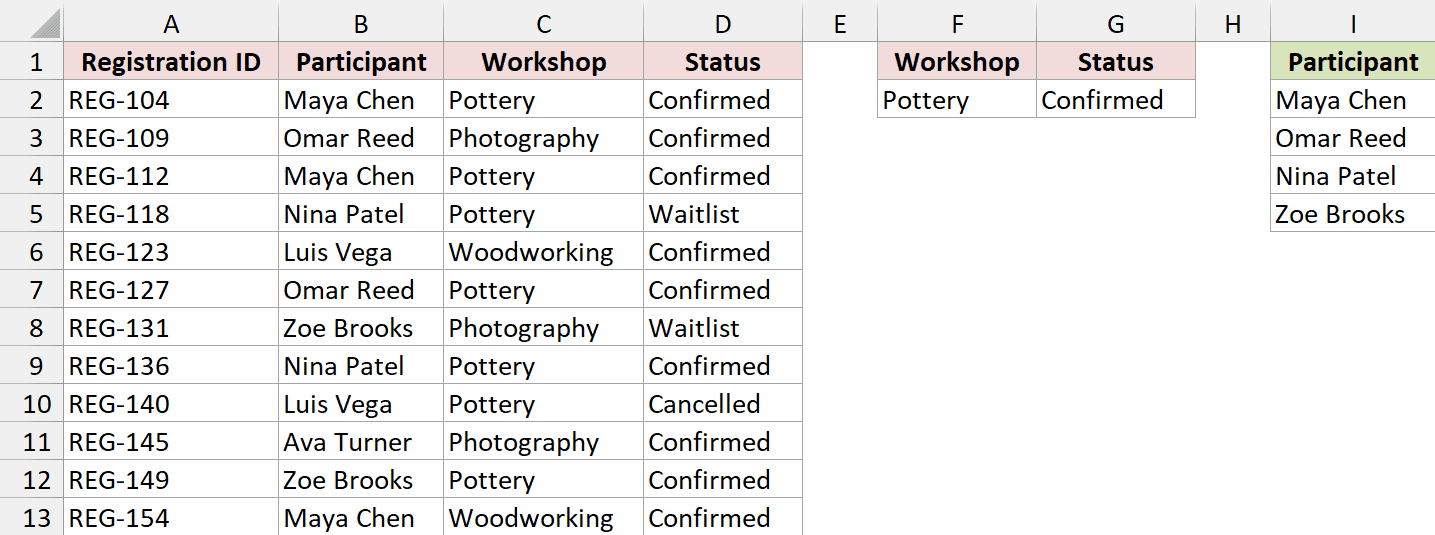
The output contains Maya Chen, Omar Reed, Nina Patel, and Zoe Brooks. Using only Participant as the output header produces the distinct name list.
Note: Advanced Filter creates a static extract. Run it again when the source or criteria change, and clear the old output first so a shorter result doesn’t leave old names underneath.
Method #3: Using Power Query
Power Query saves the filtering and duplicate-removal steps so you can rerun them with a refresh. I’ll use the Windows desktop version of Excel here.
The 3 Power Query sheet contains the registrations in an Excel Table named Registrations. I want a separate, alphabetized list of confirmed Pottery participants.
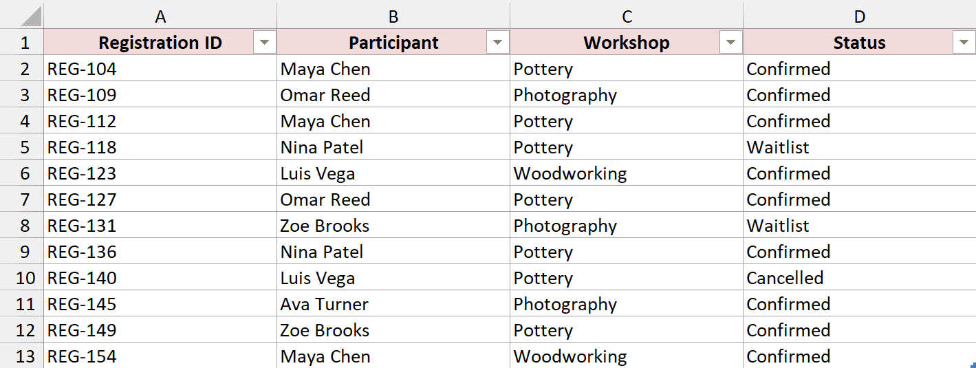
For your own data, start with an Excel Table. The example file already has the Table, completed query, and loaded result.
These steps show how to create the query from the source Table:
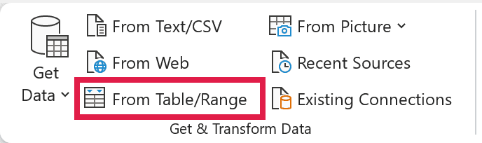
- Click a cell in the Registrations Table, then choose Data > From Table/Range to open Power Query Editor.
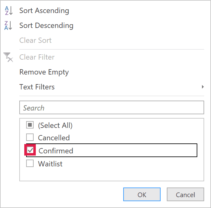
- Open the Workshop column dropdown. Clear (Select All), check Pottery, and click OK.

- Open the Status column dropdown. Clear (Select All), check Confirmed, and click OK.
Five registration rows remain, including two for Maya. Removing duplicate names will reduce the final list to four people.
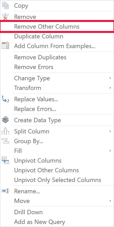
- Right-click the Participant column header and choose Remove Other Columns.
- Right-click the Participant header again and choose Remove Duplicates.
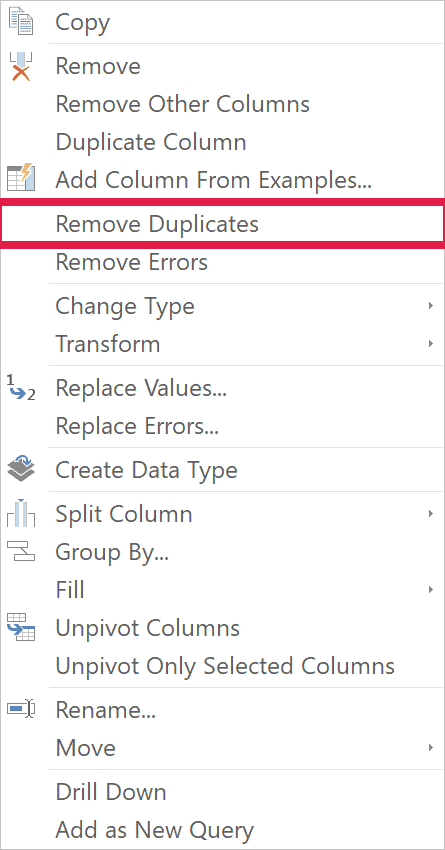
The remaining column contains just the names. Each person’s registration ID and booking details stay in the source Table.
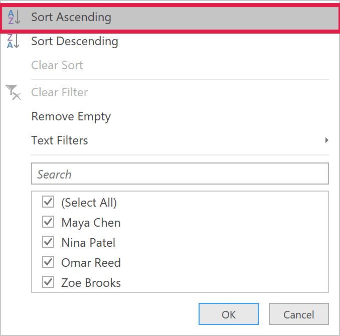
- Open the Participant dropdown and choose Sort Ascending.
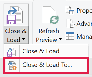
- On the Home tab, open the Close & Load dropdown and choose Close & Load To….
- In the Import Data dialog, select Table and Existing worksheet. Set the location to $F$1 on the source sheet.
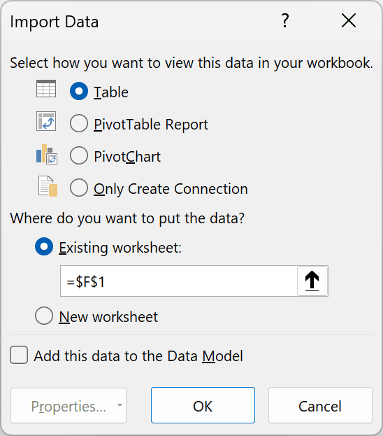
- Click OK to load the unique participant list into the worksheet.
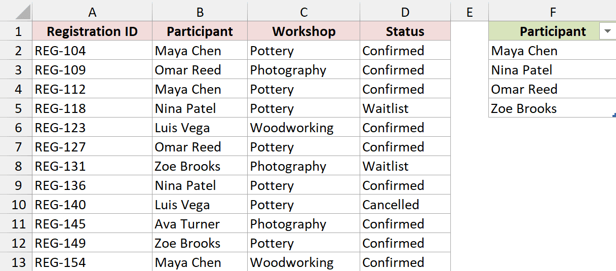
The output is Maya Chen, Nina Patel, Omar Reed, and Zoe Brooks. After adding or changing registrations in the source Table, use Data > Refresh All to update it.
Note: Power Query compares text with case sensitivity. If your source mixes names such as Maya Chen and MAYA CHEN, standardize the capitalization before removing duplicates.
Additional Notes About Unique Values With Criteria in Excel
A few details help keep your extracted list accurate:
- Keep the formula’s return range and criteria ranges the same height. B2:B13, C2:C13, and D2:D13 all cover the same registration rows.
- A blank-looking name containing spaces isn’t empty. Clean unwanted spaces in the source when names that look identical remain separate.
- A
#SPILL!error means Excel can’t place the formula’s results. Check for occupied cells, merged cells, or a formula entered inside a Table. - The download contains finished examples. Use the worksheet tabs to inspect each formula, the Advanced Filter extract, and the refreshable Power Query result.
- The formulas return lists. Counting unique values is a separate task, and the text No matches shouldn’t be counted as a participant.
Frequently Asked Questions
Here are answers to a few questions that come up when building conditional lists.
Does Unique Mean Distinct Values or Values That Appear Exactly Once?
In these examples, it means distinct values: keep one copy of every qualifying name, including names repeated in the matching rows.
UNIQUE also has an optional third argument, exactly_once. Setting it to TRUE returns only values appearing once in the array passed to UNIQUE.
When FILTER is inside UNIQUE, that test applies to the filtered rows. A name’s occurrences outside the selected group don’t affect it.
Why Do I Still See Duplicate Names When Returning Several Columns?
UNIQUE compares entire rows by default. If you pass it names alongside different registration IDs, those rows are different even when the names match.
Return just the name column when you want one row per person, as the formulas in this article do.
Does UNIQUE Follow an Ordinary Worksheet Filter?
Hiding rows or using the column-header filter doesn’t make these formulas ignore those rows. FILTER evaluates its written conditions against the referenced data.
Put the required conditions in the formula itself. A visible-rows-only list needs a different setup.
How Can the Formula Include New Registrations Automatically?
Use an Excel Table for the source and replace fixed ranges with structured column references. Table references expand when you add rows.
Keep the spill formula outside the Table. The fixed-range examples here stop at row 13, so rows added below that aren’t included automatically.
Conclusion
In this article, I showed you how to extract unique values using conditions, with formulas, Advanced Filter, and Power Query.
I hope you found this article helpful.
Other Excel articles you may also like:
