
The SUMIFS function in Excel adds values that meet your conditions, but summing several cost columns takes more than widening its sum range.
When your criteria occupy one column, SUMIFS expects a sum range with the same dimensions. You can handle this by adding separate SUMIFS results or totaling each row first.
In this article, I’ll show you both approaches, including nonadjacent columns, plus two formulas that total a block of columns without a helper.
Why SUMIFS Returns an Error With Multiple Sum Columns
A range mismatch is a common reason for a multi-column SUMIFS formula to fail.
Our service-job data has crew names in column B and labor, parts, and travel costs in columns D through F. Cell I2 contains North.
On the Range Mismatch sheet, the following formula in I6 returns #VALUE!:
=SUMIFS(D2:F11,B2:B11,I2)
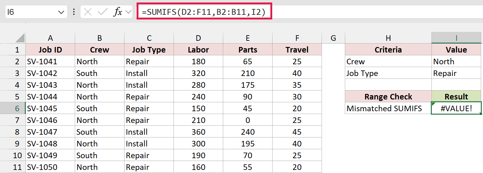
The sum range D2:F11 has ten rows and three columns. The criteria range B2:B11 has ten rows but only one column.
Microsoft’s SUMIFS documentation requires the sum range and each criteria range to have the same number of rows and columns.
Multiple criteria columns are fine when each range matches the sum range. They don’t make SUMIFS automatically repeat one crew condition across three cost columns.
Adding a separate SUMIFS for each cost column avoids this mismatch.
Method #1: Adding Multiple SUMIFS Results
I recommend this approach when you’re adding a few columns. Each SUMIFS handles one cost column, and the plus signs combine the results.
Below I have ten service jobs on the Formula Comparison sheet. Columns B and C contain the crew and job type; D, E, and F contain costs.
I want the total labor, parts, and travel costs for the North crew. North is in I2, with Repair in I3 for the second example.
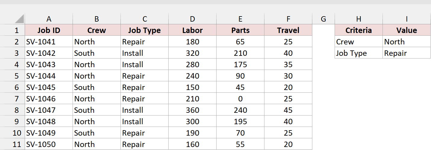
Enter this formula in I6 and press Enter:
=SUMIFS(D2:D11,B2:B11,I2)+SUMIFS(E2:E11,B2:B11,I2)+SUMIFS(F2:F11,B2:B11,I2)
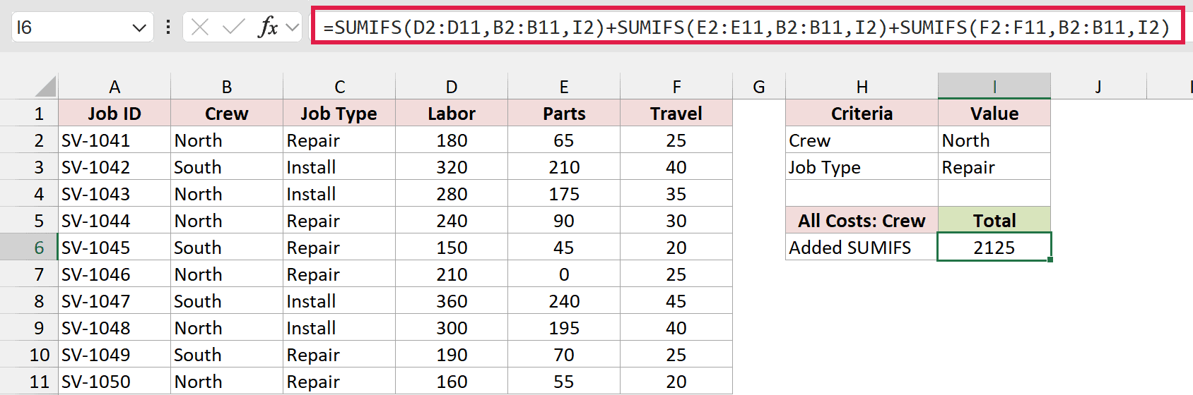
The result is 2125, covering all six North jobs.
How does this formula work?
Each SUMIFS function checks B2:B11 for the crew in I2. The three calls add matching labor, parts, and travel costs separately.
Those totals are 1370, 580, and 175. Adding them returns 2125, and every SUMIFS uses equally sized ranges.
To total only North repairs, add the job-type condition to each call. Enter this formula in I11:
=SUMIFS(D2:D11,B2:B11,I2,C2:C11,I3)+SUMIFS(E2:E11,B2:B11,I2,C2:C11,I3)+SUMIFS(F2:F11,B2:B11,I2,C2:C11,I3)
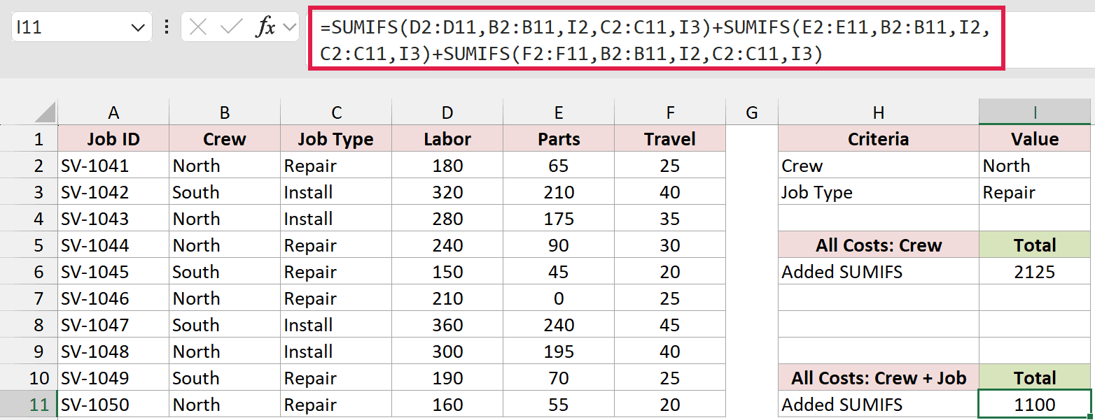
The result is 1100. SUMIFS includes a row only when its crew matches I2 and its job type matches I3.
Keep both conditions in all three calls. Leaving out the job-type condition from one call would include installation costs from that column.
Adding Nonadjacent Columns
You can also skip a cost column. On the Selected Costs sheet, I2 still contains North and I3 contains Repair.
To add labor and travel while excluding parts, enter this formula in I6:
=SUMIFS(D2:D11,B2:B11,I2,C2:C11,I3)+SUMIFS(F2:F11,B2:B11,I2,C2:C11,I3)
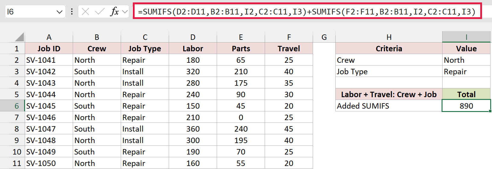
The result is 890: 790 in labor and 100 in travel. No rearranging is needed because each SUMIFS can point to a different column.
Method #2: Creating a Helper Column
If repeating SUMIFS for every cost column makes your formula too long, calculate a total for each job first.
Below I have the same service-job data on the Row Totals sheet. Columns D through F contain the three costs I want to combine.
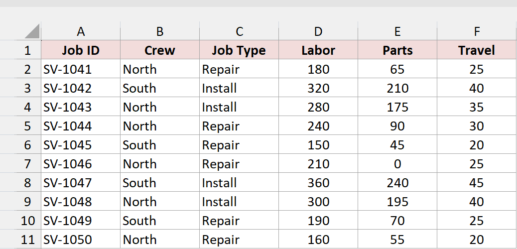
Add the heading Row Total in G1. In G2, enter the following formula, then copy it down through G11:
=SUM(D2:F2)
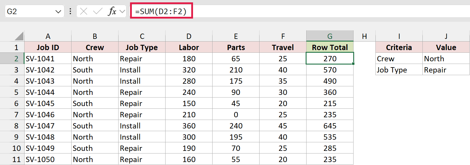
The first job totals 270: 180 for labor, 65 for parts, and 25 for travel. Each formula below G2 calculates its own row’s total.
The SUM function combines the costs within a row, leaving SUMIFS with one column to add. You can also check each job’s total in column G.
For this sheet, the criteria card is in I1:J3. Enter North in J2 and Repair in J3.
To total all North jobs, enter this formula in J6:
=SUMIFS(G2:G11,B2:B11,J2)
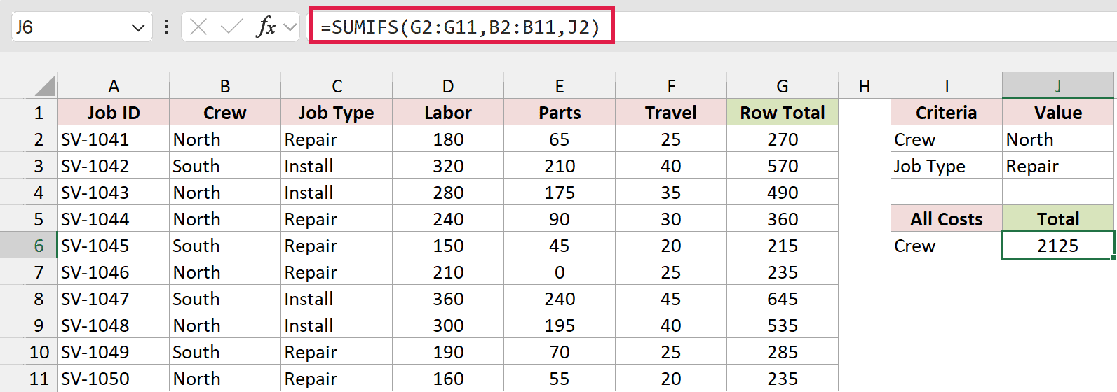
The result is 2125. SUMIFS now adds the row totals in G2:G11 wherever the crew in column B matches J2.
For North repairs only, enter this formula in J7:
=SUMIFS(G2:G11,B2:B11,J2,C2:C11,J3)
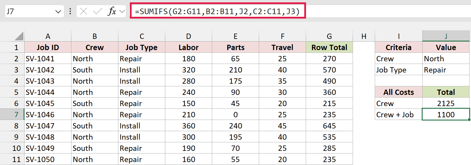
This returns 1100, matching the first method. You can add more criteria without repeating them separately for labor, parts, and travel.
Method #3: Using the SUMPRODUCT Function
If you want one formula without a helper column, SUMPRODUCT can apply a row condition across the whole cost block and add the results.
Unlike the separate SUMIFS calls, this formula uses D2:F11 as one block. It’s useful when you have many adjacent numeric columns.
Below I have the service jobs on the Formula Comparison sheet. I want the total in D2:F11 for the North crew named in I2.
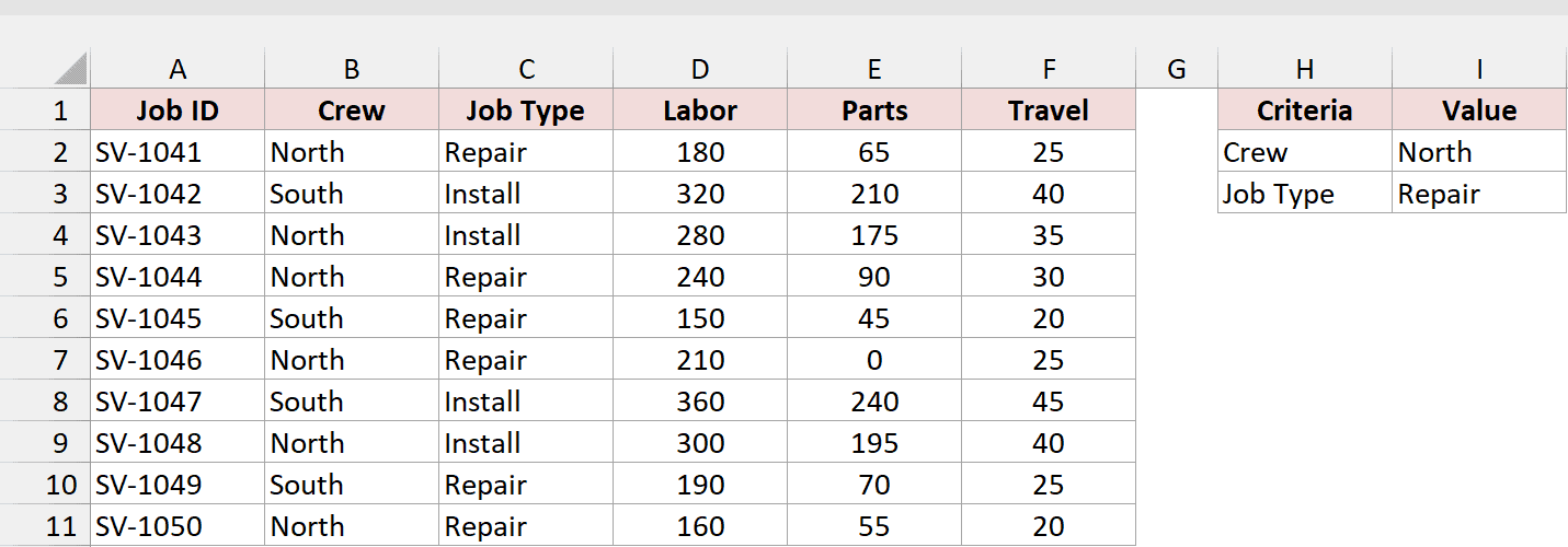
Enter this formula in I7:
=SUMPRODUCT((B2:B11=I2)*D2:F11)
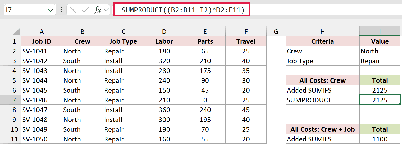
It returns 2125, matching the added SUMIFS result shown above it.
How does this formula work?
The comparison B2:B11=I2 produces TRUE for North jobs and FALSE for the others. Multiplication converts those values to 1 and 0.
Excel applies each row’s 1 or 0 across its three costs. North costs remain unchanged, South costs become zero, and SUMPRODUCT adds the resulting values.
The multiplication happens inside one expression. Keep the asterisk as shown; replacing it with a comma changes how SUMPRODUCT receives the arrays.
For North repairs, enter this formula in I12:
=SUMPRODUCT((B2:B11=I2)*(C2:C11=I3)*D2:F11)
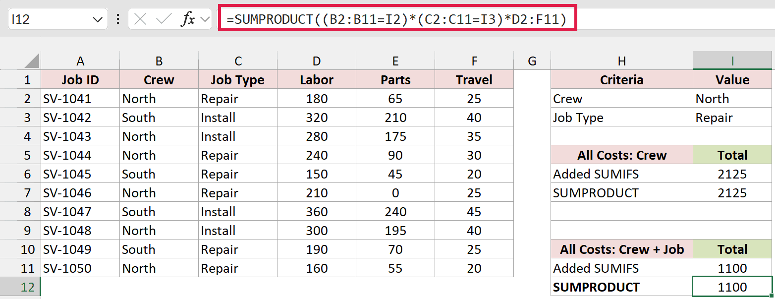
The result is 1100. Multiplying the two conditions keeps a row only when both comparisons are TRUE.
Press Enter normally for these formulas. You don’t need Ctrl+Shift+Enter.
Note: Keep the cost block numeric. With this multiplication-based formula, text such as pending in D2:F11 causes #VALUE!. Genuine empty cells work, but text needs cleaning first.
Use bounded ranges such as D2:F11 instead of entire columns. That avoids calculating over hundreds of thousands of unused rows.
Method #4: Combining SUM and FILTER
For Excel 365, Excel 2021, and Excel 2024, FILTER provides another way to collect the matching costs before adding them.
FILTER selects rows that meet your condition. Wrapping it in SUM adds all the numbers in those rows, including values across several columns.
Below I have the service jobs on the Formula Comparison sheet. The costs are in D2:F11, with North in I2 and Repair in I3.
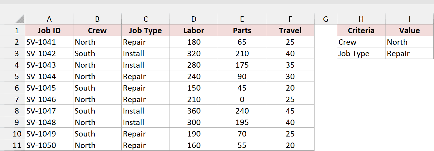
To add all costs for North, enter this formula in I8:
=SUM(FILTER(D2:F11,B2:B11=I2,0))
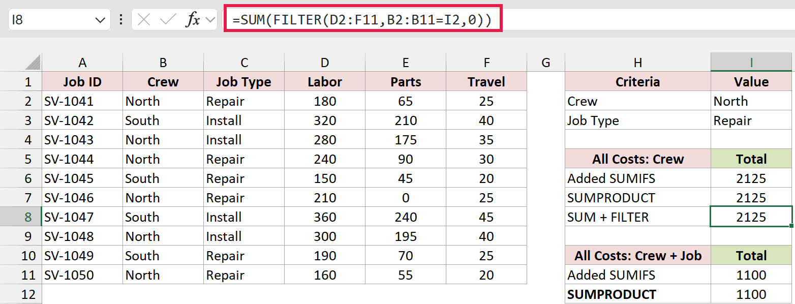
The result is 2125, matching the other two formulas in the comparison.
How does this formula work?
FILTER keeps all three cost columns for rows where the crew matches I2. SUM then adds the filtered numbers and returns one total.
The final 0 is FILTER’s if_empty argument. If no crew matches, FILTER returns zero, so the combined formula also returns zero instead of a no-match error.
Although FILTER can spill a table into neighboring cells, SUM reduces its output here to a single value. You don’t need a separate spill area.
To total North repairs, enter this formula in I13:
=SUM(FILTER(D2:F11,(B2:B11=I2)*(C2:C11=I3),0))
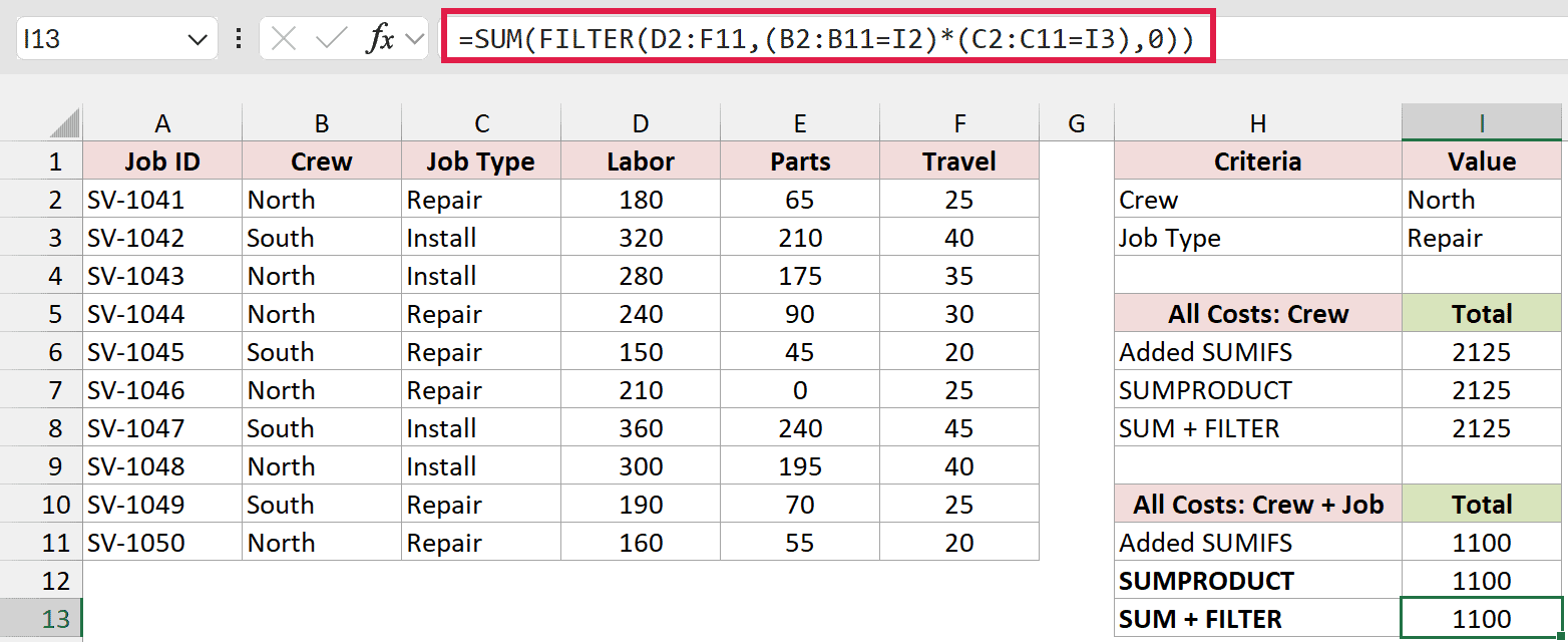
This returns 1100. Multiplying the conditions tells FILTER to keep only rows that match both North and Repair.
FILTER isn’t available in Excel 2016 or Excel 2019. Use one of the first three methods if your version doesn’t support it.
Additional Notes About Summing Multiple Columns in Excel
All four methods solve the same task. Here’s how I’d choose between them for a new worksheet.
| Approach | When to Use It | Excel Versions Covered |
|---|---|---|
| Add SUMIFS results | A few columns, especially nonadjacent ones | 2016, 2019, 2021, 2024, Microsoft 365 |
| Helper column + SUMIFS | You also want a visible total for every row | 2016, 2019, 2021, 2024, Microsoft 365 |
| SUMPRODUCT | Many adjacent numeric columns without a helper | 2016, 2019, 2021, 2024, Microsoft 365 |
| SUM + FILTER | You prefer to filter matching rows, then total them | 2021, 2024, Microsoft 365 |
For just two or three columns, I’d start with added SUMIFS results. The separate ranges make it clear which costs are included.
Keep these details in mind when adapting the examples:
- Keep every criteria range aligned to the same data rows. Equal sizes alone won’t fix ranges that start on different rows.
- Exclude headers and existing total rows from the cost ranges, or you may get errors or double-count values.
- These examples use AND logic: a job must match both crew and job type when both conditions appear.
- Adding new rows below row 11 requires extending every relevant range. The workbook’s formulas use fixed ranges.
- Excel installations that use semicolons as argument separators need semicolons in place of the formulas’ commas.
Numbers stored as text also deserve a check. In these examples, SUMIFS and SUM ignore text costs, even when they look like numbers.
The multiplication in the SUMPRODUCT formulas can convert numeric text to numbers, so it can produce a different total. Convert your cost columns to real numbers for consistent results.
The download contains completed formulas on Formula Comparison, Row Totals, and Selected Costs. The Range Mismatch sheet deliberately retains #VALUE! to demonstrate the incompatible ranges.
Frequently Asked Questions
These details can matter when you adapt the formulas to your own report.
Can I Use Wildcards in the Criteria?
Yes, SUMIFS supports * for any sequence of characters and ? for one character. Put a wildcard pattern in the criteria cell to use partial matches.
The equality comparisons in the SUMPRODUCT and FILTER examples don’t interpret those wildcards. Their conditions would need a different text-matching expression.
Do These Formulas Include Filtered-Out Rows?
Yes. Hiding rows or applying a worksheet filter doesn’t remove them from these calculations. The formulas apply their own criteria to all referenced rows.
The FILTER function also evaluates its include condition independently of the worksheet’s filter buttons.
Can I Use Excel Tables So New Jobs Are Included?
Yes. Convert the source data to an Excel Table and replace the fixed ranges with structured references to its columns.
Those references adjust as table rows are added. Keep summary formulas outside the source table, and keep totals rows out of the data being added.
Conclusion
In this article, I showed you how to sum multiple columns with SUMIFS, including two conditions and nonadjacent columns, plus helper-column, SUMPRODUCT, and FILTER approaches.
I hope you found this article helpful.
Other Excel articles you may also like:
