How to Use Structured References in Excel

Structured references in Excel let a formula use a Table’s name and column headers, like Sales[Amount], instead of cell addresses such as C2:C9.

They make formulas easier to read. They also grow with the Table, so a new row gets picked up without you editing a single range.

The catch is that they only work with a real Excel Table, and the syntax has a few quirks.

There’s the @ sign, the double brackets, and a surprise when you drag a formula sideways.

In this article, I’ll show you how to write current-row references, use Table columns in SUMIFS and XLOOKUP, lock a reference so it doesn’t shift, and read the Total Row.

Create the Table First

Every method below needs a real Excel Table, not a range with colored headers. So let’s set that up first.

Below I have an equipment rental register with a Rental ID, the Equipment, its Status, the Daily Rate, and the number of Days rented.

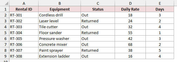
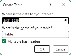
Here are the steps to turn it into a Table and give it a name:

1. Click any cell in the data and press Ctrl + T. In the Create Table dialog, keep My table has headers checked and click OK.

2. On the Table Design tab, click in the Table Name box, type GearIssues, and press Enter.

Excel names a new Table Table1, Table2, and so on. A name that says what’s in the Table makes every formula below much easier to read.

Method #1: Using @ References in a Calculated Column

A calculated column is a Table column where one formula runs on every row. It’s where you’ll use structured references most, and Excel writes them for you as you click.

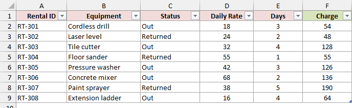
Below I have the GearIssues Table with an empty Charge column. I want Charge to be the Daily Rate multiplied by the Days for each rental.

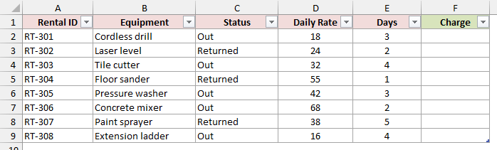
Here are the steps to create the formula by pointing and clicking:

1. Click cell F2, type an equal sign (=), click D2, type an asterisk (*), and then click E2.

2. Press Enter. Excel fills the formula down the whole Charge column.

Here is the formula Excel writes in F2:

=[@[Daily Rate]]*[@Days]

How does this formula work?

The @ sign means “this row”. So [@Days] is the Days value in the same row as the formula.

Daily Rate gets an extra pair of brackets because its header has a space in it. Days is a single word, so it doesn’t need them.

For RT-301, that’s 18 times 3, which returns 54. Every other row gets its own charge, and you never had to drag the formula down.

Method #2: Using Table Column References in SUM and COUNTIF

Inside the Table, you use @ for the current row. Outside the Table, you refer to a whole column by putting the Table name in front of the header.

Below I have the same GearIssues Table on the Gear Issues sheet. I want the total of the Charge column and a count of the rentals that are still Out.

Here is the formula for the total charge in H2:

=SUM(GearIssues[Charge])

GearIssues[Charge] means every data cell in the Charge column. The header isn’t included, so SUM adds the eight charges and returns 801.

And here is the formula in I2 that counts the rentals still marked Out:

=COUNTIF(GearIssues[Status],"Out")

COUNTIF checks every Status in the Table and returns 5.

These references also keep up when the Table grows. Say a new rental comes in: RT-309, a Shop vacuum at 22 a day for 2 days.

Type it in the row right below the Table and the Table grows to include it. The Charge formula fills in by itself, and both summary formulas update.

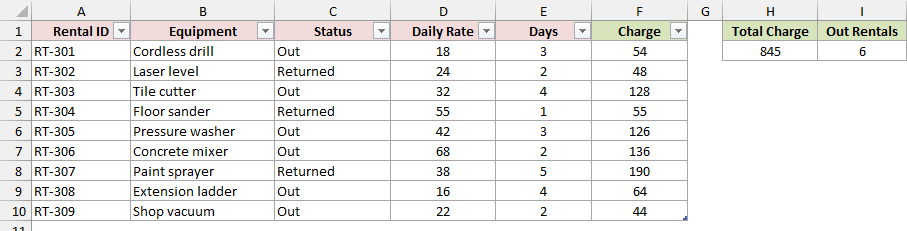
The total goes from 801 to 845 and the count goes from 5 to 6, without you editing either formula.

Method #3: Using Structured References in SUMIFS and XLOOKUP

Structured references work inside any function that takes a range. Conditional sums and lookups are where they read best.

Below I have the GearIssues Table next to the total and count from the previous method.

I want the total charge for rentals that are Out, and the charge for rental RT-305.

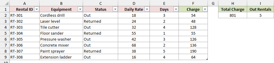
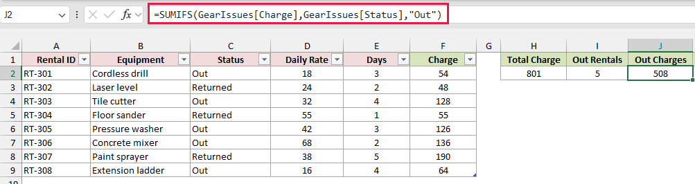
Here is the SUMIFS formula in J2:

=SUMIFS(GearIssues[Charge],GearIssues[Status],"Out")

How does this formula work?

GearIssues[Charge] is the column to add up, GearIssues[Status] is the column to check, and “Out” is the condition. The five Out rentals add up to 508.

Here is the XLOOKUP formula in K2:

=XLOOKUP("RT-305",GearIssues[Rental ID],GearIssues[Charge])

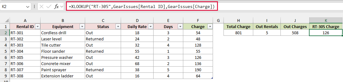
It looks for RT-305 in the Rental ID column and returns the matching value from the Charge column, which is 126.

Note: XLOOKUP is available in Microsoft 365 and Excel 2021 or later. In older versions, =VLOOKUP(“RT-305”,GearIssues,6,FALSE) returns the same 126, using the Table name as the lookup range.

Method #4: Using a Column Range in the Current Row

Sometimes you need several side-by-side columns from the same row, not just one. A colon between two column names gives you that range.

Below I have a second Table, WeeklyUsage, on the Weekly Usage sheet.

It shows how many days each item was rented in each of four weeks, and I want the Total Days in column F.

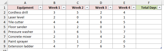
Here is the formula in F2:

=SUM(WeeklyUsage[@[Week 1]:[Week 4]])

How does this formula work?

[Week 1]:[Week 4] means every column from Week 1 through Week 4. The @ in front keeps it to the current row.

So for the Cordless drill, it adds 3, 5, 2, and 4 and returns 14. Since it’s a calculated column, the rest of the rows fill in automatically.

Method #5: Locking a Structured Reference (Absolute Reference)

Structured references don’t use dollar signs, so you can’t lock them the usual way. That becomes a problem as soon as you drag one sideways.

Below I have the GearIssues Table with a small summary under it in A11:C13. I want the Total Days and Total Charge for each Status.

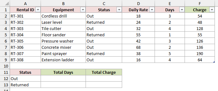
Here’s the formula I’d start with in B12:

=SUMIFS(GearIssues[Days],GearIssues[Status],$A12)

It works in B12 and returns 16. But drag it right to C12 and down to row 13, and here’s what C12 ends up with:

=SUMIFS(GearIssues[Charge],GearIssues[Daily Rate],$A12)

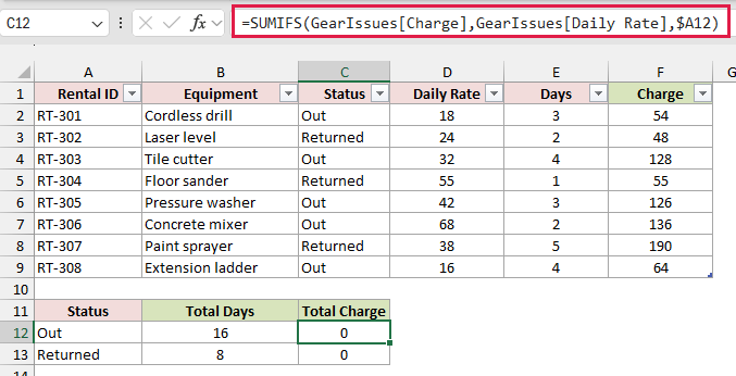
When you drag a structured reference sideways, Excel moves every column name one column over, just like a relative reference.

Days became Charge, which is what we wanted. But Status also became Daily Rate, so the condition checks the wrong column and C12 returns 0.

The fix is to write the column you want to lock as a range of just that one column: [[Status]:[Status]].

Here is the fixed formula in B12:

=SUMIFS(GearIssues[Days],GearIssues[[Status]:[Status]],$A12)

Now drag it right and down again. Here is what C12 holds this time:

=SUMIFS(GearIssues[Charge],GearIssues[[Status]:[Status]],$A12)

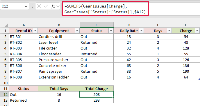
Days moved over to Charge, but Status stayed put. The Out rentals come to 16 days and 508 in charges, and the Returned rentals come to 8 days and 293.

Note: The shift only happens when you drag or fill a formula. If you copy the cell with Ctrl + C and paste it with Ctrl + V, the column names stay exactly as they are.

Method #6: Using the Total Row and #Totals

A Table can also carry its own Total Row. Once it’s on, you can point to it from anywhere with #Totals.

Below I have the WeeklyUsage Table with the Total Days column filled in. I want a total for every week, plus the grand total in a cell outside the Table.

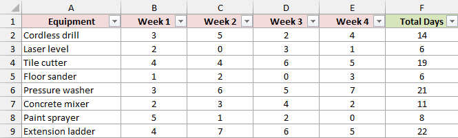
Here are the steps to turn on the Total Row:

1. Click any cell in the Table, go to the Table Design tab, and check the Total Row box.

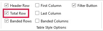
Excel adds a Total row at the bottom and totals the last column for you.

For the week columns, click the Total cell under each one, open its drop-down, and pick Sum.

Here is the formula Excel puts in F10:

=SUBTOTAL(109,[Total Days])

How does this formula work?

SUBTOTAL with 109 adds up only the visible rows, so the total follows any filter you apply. It returns 107, and the weeks come to 24, 28, 28, and 27.

[Total Days] needs no Table name here because the formula sits inside the Table.

Here is the formula in H2 that pulls the grand total from outside the Table:

=WeeklyUsage[[#Totals],[Total Days]]

The #Totals part points to the Total row, and [Total Days] picks the column, so this returns 107. It needs the Total Row turned on to have something to point to.

Structured Reference Cheat Sheet

Here’s every form from this article in one place. The Cheat Sheet tab in the example file has most of them with live formulas you can click on.

Reference	What It Refers To	Result in the Example
[@Days]	Days in the same row (inside the Table)	3 for RT-301
GearIssues[Charge]	Every data cell in the Charge column	SUM returns 801
GearIssues	All data rows, without the headers	ROWS returns 8
GearIssues[#Data]	Same as the Table name on its own	ROWS returns 8
GearIssues[#Headers]	The header row only	COUNTA returns 6
GearIssues[#All]	Headers, data, and the Total Row if shown	ROWS returns 9
GearIssues[[Daily Rate]:[Days]]	Adjacent columns from Daily Rate to Days	COLUMNS returns 2
WeeklyUsage[@[Week 1]:[Week 4]]	Week 1 through Week 4 in the same row	SUM returns 14 for the Cordless drill
GearIssues[[Status]:[Status]]	The Status column, locked when dragged	COUNTIF of “Out” returns 5
WeeklyUsage[#All]	Includes the Total Row when it’s on	ROWS returns 10
WeeklyUsage[[#Totals],[Total Days]]	One cell of the Total Row	Returns 107

Additional Notes About Structured References in Excel

• If a header contains #, [, ], ‘, or @, put an apostrophe before that character. A header called Item # in a Table named Parts becomes Parts[Item '#]. Without the apostrophe, Excel rejects the formula.
• Don’t want Excel writing Table names when you click cells? Go to File > Options > Formulas and uncheck Use table names in formulas.
• If you convert a Table back to a normal range (Table Design > Convert to Range), Excel rewrites every structured reference as a regular absolute address, like $F$2:$F$9.
• Tables and structured references work in Excel 2007 and later, and the @ shorthand has been around since Excel 2010.

Frequently Asked Questions

Here are answers to a few common questions about using structured references.

Why does Excel change #This Row to @ in my formula?

The @ sign is the short form of [#This Row].

If you type GearIssues[[#This Row],[Daily Rate]], Excel converts it to [@[Daily Rate]] as soon as you press Enter. Both point to the same cell.

What happens to structured references when I rename a Table or a column?

Excel updates them for you. Rename the Charge column to Fee, and =SUM(GearIssues[Charge]) becomes =SUM(GearIssues[Fee]).

The exception is a reference typed as text inside INDIRECT, like INDIRECT("GearIssues[Charge]"). That text doesn’t change, so it returns a #REF! error.

Can a structured reference point to a Table in another workbook?

Yes. The source workbook needs to be open, though. If it’s closed when Excel recalculates, the formula returns a #REF! error.

Why can’t I use a structured reference in Data Validation or Conditional Formatting?

Both dialogs reject structured references typed directly. For a drop-down list, use =INDIRECT("GearIssues[Status]") as the source instead.

For a conditional formatting rule, use a normal cell reference, like =$C2="Out".

Conclusion

Structured references take a little getting used to, but they make formulas easier to read and keep them working as your data grows.

For most work, the @ references in a calculated column and the Table-name references in SUM, SUMIFS, and XLOOKUP are all you’ll need.

Keep the [[Status]:[Status]] trick handy for the day a dragged formula suddenly returns 0.

I hope you found this article helpful.

Other Excel articles you may also like:

• XLOOKUP vs VLOOKUP in Excel
• How to Sum a Column in Excel?
• How to Use SUMIFS with INDEX MATCH in Excel
• How to Create a Dynamic Named Range