How to Calculate Median in an Excel Pivot Table

A median gives you a typical value for your Excel PivotTable summary without letting one extreme number pull it around.

You’ll find Sum, Average, Count, and other summaries in Value Field Settings, but there’s no Median option.

You can use a DAX measure inside the PivotTable or a MEDIAN IF formula beside it.

I’ll also show you GROUPBY and PIVOTBY, Microsoft 365 formulas that build a PivotTable-style summary.

Method #1: Using a DAX Measure in the Data Model

I recommend a DAX measure when you want the median inside the PivotTable itself. You can’t put a real median there with the regular summary options.

You can write a small DAX formula, called a measure, in the Data Model. You then use it in your PivotTable like a field.

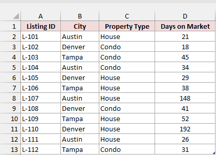
Below I have a dataset of 12 home listings in an Excel Table named HomeListings, with Listing ID, City, Property Type, and Days on Market.

I want each city’s median inside the PivotTable.

If your data isn’t a Table yet, select any cell, press Ctrl + T, and click OK.

Then type HomeListings in the Table Name box on the Table Design tab.

You can create the PivotTable and its measure with these steps:

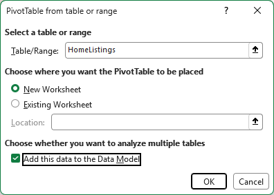
1. Select any cell in the table. On the Insert tab, click PivotTable. Microsoft 365 calls the dialog “PivotTable from table or range”; older versions call it “Create PivotTable”. Keep New Worksheet selected. Check “Add this data to the Data Model” and click OK.

2. Go to the Power Pivot tab, click Measures, then choose New Measure.

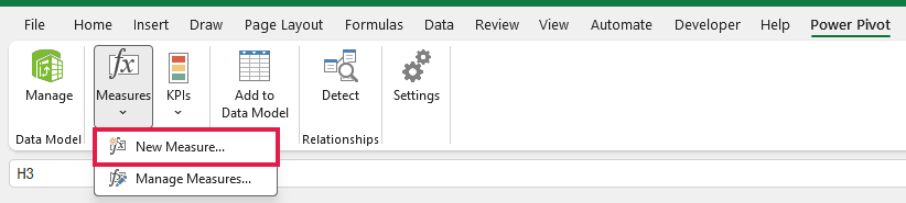
Note: If you don’t have a Power Pivot tab, right-click HomeListings in the PivotTable Fields pane and choose Add Measure. It opens the same Measure dialog.

3. In the Measure dialog, keep HomeListings as the Table name. Type Median Days on Market as the Measure name. In the Formula box, replace the entire contents, including the existing equal sign, with the formula below. Then click OK. You can leave Formatting Options on General because you’re returning plain numbers.

=MEDIAN(HomeListings[Days on Market])

4. In the PivotTable Fields pane, check City to put it in Rows. Check your new Median Days on Market measure to put it in Values.

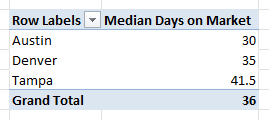
Under Row Labels and Median Days on Market, you get Austin 30, Denver 35, Tampa 41.5, and Grand Total 36.

How does this formula work?

I use MEDIAN in this measure. It reads Days on Market for the current PivotTable row, so Austin’s row uses only Austin’s listings.

MEDIAN sorts the numbers and returns the middle value. With an even count, it returns the average of the two middle values.

Austin’s listings took 21, 26, 34, and 148 days. MEDIAN averages the middle pair, so (26 + 34) / 2 returns 30.

In Grand Total, the measure runs over all 12 listings. It returns 36, the median of all listings rather than the median of the three city medians.

You can also break the median down by property type with one more step:

5. Drag Property Type into the Columns area of the PivotTable Fields pane.

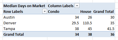
You get medians by city and property type, with overall totals of 34 for condos, 38 for houses, and 36 for all listings.

Denver’s house median is 110.5 days. There are only two houses, at 29 and 192 days, so MEDIAN averages those two values.

You need Excel for Windows with Power Pivot / the Data Model (Excel 2016 or later, including Microsoft 365).

Excel for Mac can’t create Data Model measures, so use Method #2 or #3.

Your median responds to PivotTable filters and slicers. After changing your source data, refresh the PivotTable to update the median.

Method #2: Using MEDIAN and IF Next to a Pivot Table

You can keep a regular PivotTable and calculate the median beside it instead. You don’t need the Data Model, and you can use this approach in every Excel version.

Below I have a dataset of 12 home listings in A1:D13, with Listing ID, City, Property Type, and Days on Market.

I want each city’s median beside a PivotTable.

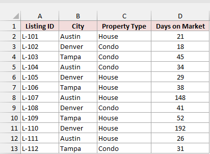
First, you can build a regular PivotTable with these steps:

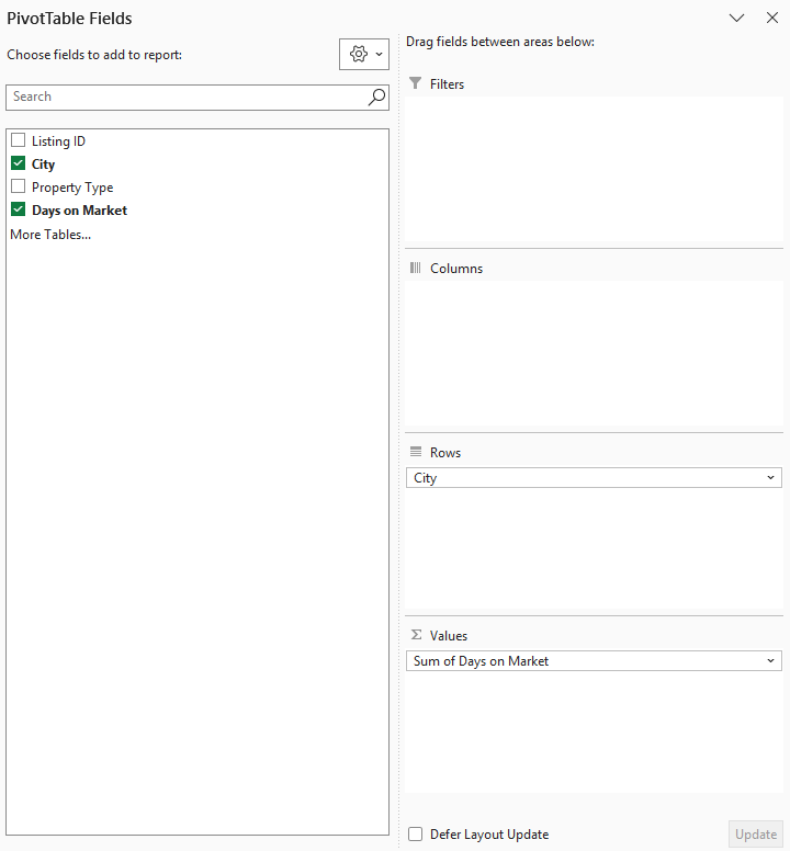
1. Select any cell in the data. On the Insert tab, click PivotTable. Choose Existing Worksheet, set Location to F1 on the same sheet, and click OK. In the PivotTable Fields pane, check City for Rows and Days on Market for Values. You’ll see Sum of Days on Market in Values.

2. Right-click any number in the PivotTable and choose Value Field Settings. Look at the “Summarize value field by” list, choose Average, and click OK.

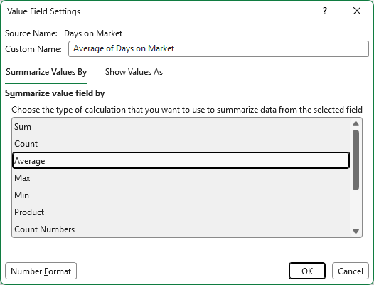
You can choose several summaries in that list, including:

• Sum
• Count
• Average
• Max
• Min
• Product

You won’t find Median among them.

You now have Average of Days on Market in F1:G5.

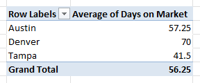
You get averages of 57.25 for Austin, 70 for Denver, and 41.5 for Tampa, with 56.25 in Grand Total.

The 148-day and 192-day listings raise the averages for Austin and Denver. Tampa’s average and median are both 41.5.

Now you can add the median beside the PivotTable:

3. In H1, type Median Days on Market. Enter the formula below in H2, then copy it down to H4. For the Grand Total row, enter =MEDIAN($D$2:$D$13) in H5 because “Grand Total” isn’t a city.

=MEDIAN(IF($B$2:$B$13=F2,$D$2:$D$13))

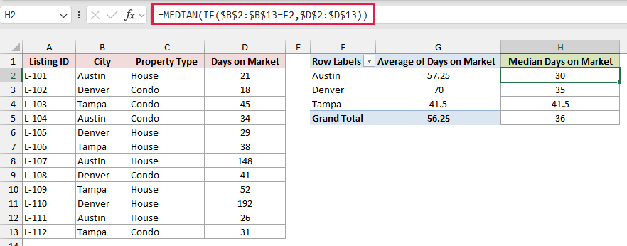
I use one formula per city row here because each copy reads that row’s city label from the PivotTable.

You get 30, 35, and 41.5 in H2:H4. In H5, you get 36 for all listings.

How does this formula work?

I use $B$2:$B$13=F2 to compare each City cell with the city in F2. The comparison returns TRUE for Austin’s rows and FALSE for the others.

IF keeps the Days on Market value wherever that comparison returns TRUE and returns FALSE everywhere else.

I use MEDIAN on those results. It ignores FALSE and returns the middle of the remaining numbers, or 30 for Austin.

I lock the source ranges with $ so they stay put when you copy down. You leave F2 relative so it changes to F3 and F4.

Note: In Excel 2019 and older, press Ctrl + Shift + Enter after typing the formula. In Microsoft 365 and Excel 2021 or later, you can press Enter.

This median is calculated outside the PivotTable. The formula reads the source data directly, so it ignores PivotTable filters and slicers.

The formula uses fixed ranges ($B$2:$B$13 and $D$2:$D$13), so extend them if you add rows.

If a new city appears after refreshing, copy the formula down to it and move the Grand Total formula to the new Grand Total row.

Method #3: Using the GROUPBY and PIVOTBY Functions

You can also skip the PivotTable and build its style of summary with a formula.

In Microsoft 365, you can pass MEDIAN directly to GROUPBY or PIVOTBY.

These formulas update automatically when your data changes, without refreshing.

Below I have a dataset of 12 home listings in A1:D13, with Listing ID, City, Property Type, and Days on Market.

I want a formula summary of each city’s median.

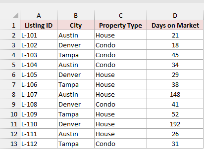
In F1, type City. In G1, type Median Days on Market. Then enter this formula in F2:

=GROUPBY(B2:B13,D2:D13,MEDIAN)

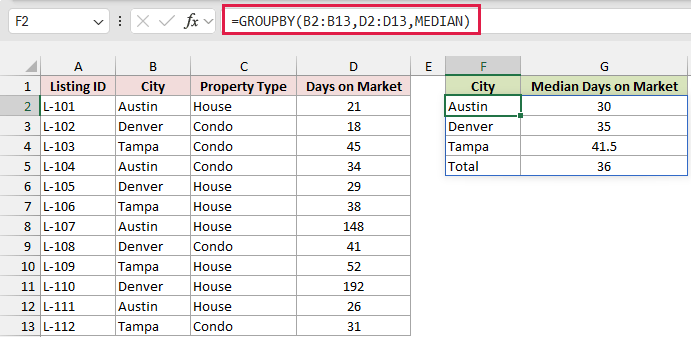
You get Austin 30, Denver 35, Tampa 41.5, and Total 36.

How does this formula work?

I give GROUPBY three arguments:

• I group by the City column, B2:B13.
• I summarize Days on Market, D2:D13.
• I calculate the median with MEDIAN. You type it without parentheses because you’re passing the function itself.

Excel adds a Total row automatically. Like the DAX measure, GROUPBY calculates the median of all 12 listings there.

You can add property types as columns with PIVOTBY. Place it next to the GROUPBY result, leaving column H empty between them.

In I1, enter this formula:

=PIVOTBY(B2:B13,C2:C13,D2:D13,MEDIAN)

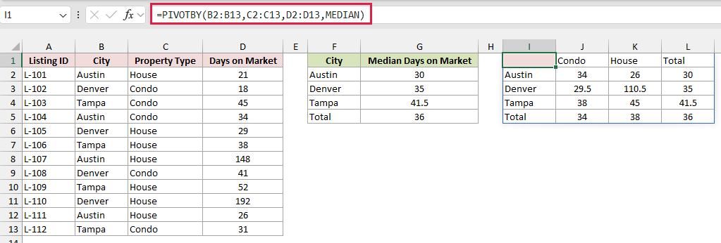
You get the same city and property type medians as in the Data Model PivotTable, with Total labels.

I pass Property Type, C2:C13, as the second argument. PIVOTBY uses it for the columns and otherwise summarizes the data like GROUPBY.

You need to leave room below and to the right of both formulas because their results spill into neighboring cells.

Additional Notes About Calculating Median in an Excel Pivot Table

You can avoid a few misleading results by keeping these points in mind:

• MEDIAN IF counts a blank in a matching row as 0. If Austin’s 34 days for L-104 were blank, MEDIAN IF would return 23.5 instead of 26. To exclude blanks, use =MEDIAN(IF(($B$2:$B$13=F2)*($D$2:$D$13<>""),$D$2:$D$13)). GROUPBY and the DAX MEDIAN measure skip blanks.
• The Grand Total median is the median of all values, rather than the median or average of group medians. Here, you get 36 overall; the median of the three city medians would be 35.
• You can also calculate a median per group in Power Query. Under Home > Group By, choose the Median operation. You get a summary table rather than a PivotTable.
• Medians and averages may be similar without extreme values, as they are for Tampa. Larger outliers pull the average further from the typical value, making the median more useful.

Frequently Asked Questions

Here are answers to a few questions you might have.

Can I Use a Calculated Field to Get the Median in a Pivot Table?

No. You can’t use a calculated field because it works on summed field values, rather than the individual rows you need for a median. Use a DAX measure instead.

Why Does My Data Model Median Show Blank Cells?

This happens when numbers in your source column are stored as text. The Data Model then treats the whole column as text, so MEDIAN can’t calculate it.

Convert the column to real numbers, then refresh the PivotTable.

Can I Show the Median and the Average in the Same Pivot Table?

Yes, with the Data Model PivotTable from Method #1.

Also drag Days on Market into the Values area. Right-click it, choose Value Field Settings, and pick Average.

Average of Days on Market appears next to your Median Days on Market measure.

Conclusion

I’d choose the DAX measure when you need the median inside your PivotTable.

You can use MEDIAN IF in any Excel version, or choose GROUPBY and PIVOTBY for the quickest formula summary in Microsoft 365.

Other Excel articles you may also like:

• How to Show Percentage of Total in an Excel Pivot Table
• List.Median Function (Power Query M)
• Mean Median Mode Calculator
• How to Calculate Monthly Averages in Excel