
Monthly averages in Excel help you spot trends hidden among individual daily records, such as a change in your typical calories burned per workout.
Each average combines the records from one month, so you can compare months even when they contain different numbers of entries.
The key is to match both the month and year, keeping January from one year separate from January in another.
I’ll show you how to calculate monthly averages with two formula methods, a PivotTable, and Power Query.
Method #1: Using AVERAGEIFS and EOMONTH
AVERAGEIFS averages values that meet your conditions. Here, I’ll use two date conditions to include only the workouts within each month.
This is the method I’d reach for first. It works in all modern Excel versions and recalculates when you change the source values.
Below I have a log of 12 workouts, with workout dates and calories burned, and I want the average calories burned for each month.
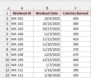
Workout ID is in column A, Workout Date in B, and Calories Burned in C. The data runs from row 2 to row 13.
The workouts span October 2025 to January 2026. I’ll put the monthly summary beside the log, leaving column D empty as a spacer.
Type Month in E1. In E2:E5, enter the first day of each month in your regional date format (the dates shown use US month/day/year):
- E2:
10/1/2025 - E3:
11/1/2025 - E4:
12/1/2025 - E5:
1/1/2026
Use real dates here, rather than text such as “October.” The formula needs a date to build the start and end of each month’s range.
Apply the custom number format mmm yyyy to E2:E5. You’ll see Oct 2025, Nov 2025, Dec 2025, and Jan 2026, while the underlying values remain dates.
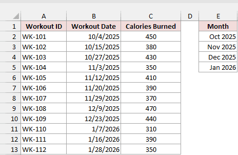
Type Average Calories in F1. Enter this formula in F2, then copy it down to F5:
=AVERAGEIFS($C$2:$C$13,$B$2:$B$13,">="&E2,$B$2:$B$13,"<="&EOMONTH(E2,0))
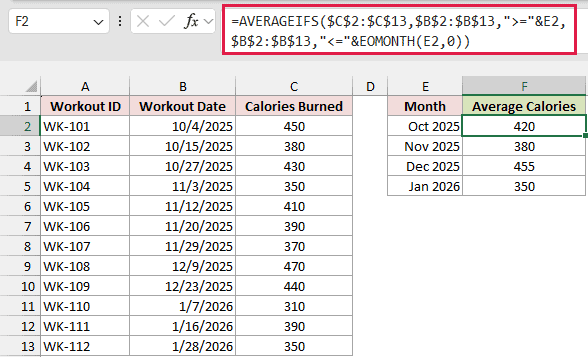
You’ll get 420 for October, 380 for November, 455 for December, and 350 for January in F2:F5.
How does this formula work?
I ask AVERAGEIFS to average the calories in $C$2:$C$13, using the workout dates in $B$2:$B$13 to decide which rows qualify.
The first condition, ">="&E2, includes dates on or after the first day of the month in E2. For October, that starts at October 1, 2025.
The second condition, "<="&EOMONTH(E2,0), includes dates on or before the last day of that month.
EOMONTH returns the month’s final date. With October 1, 2025 in E2, it returns October 31, 2025. The 0 tells it to use the same month.
The dollar signs keep both source ranges fixed when you copy the formula. E2 remains relative, so it changes to E3, E4, and E5.
Because you’re comparing full dates, October 2025 stays separate from October in any other year.
Method #2: Using the GROUPBY Function
If you’re using Microsoft 365, you can build the entire monthly summary with one formula instead of creating a month list first.
GROUPBY collects rows with the same label and calculates a result for each group. I’ll give it a year-month label and ask it to average the calories.
Below I have a log of 12 workouts, with workout dates and calories burned, and I want the average calories burned for each month.
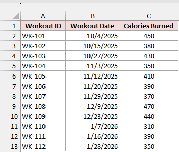
Workout ID is in column A, Workout Date in B, and Calories Burned in C. The data runs from row 2 to row 13.
Type Month in E1 and Average Calories in F1, leaving column D empty. Keep E2:F5 clear so the formula has room for its results.
Enter this formula in E2:
=GROUPBY(TEXT(B2:B13,"yyyy-mm"),C2:C13,AVERAGE,0,0)
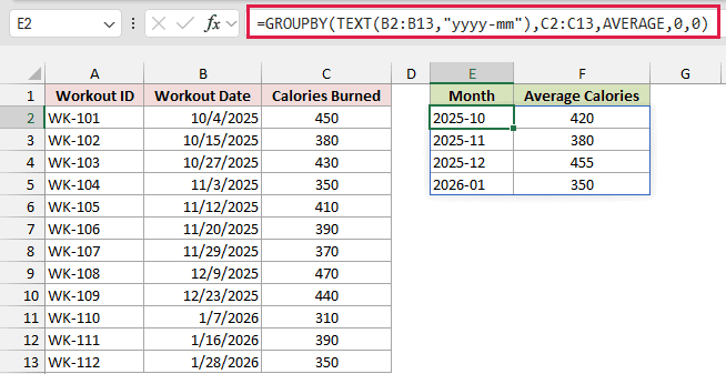
The formula spills into E2:F5 automatically, pairing each month with its average:
- 2025-10: 420
- 2025-11: 380
- 2025-12: 455
- 2026-01: 350
How does this formula work?
First, TEXT(B2:B13,"yyyy-mm") turns each workout date into a label such as 2025-10. GROUPBY puts rows with matching labels into the same group.
Next, C2:C13 supplies the calories you want to summarize. AVERAGE tells GROUPBY which calculation to apply to each month’s group.
You pass the function name AVERAGE itself, without parentheses after it.
The fourth argument, 0, tells GROUPBY that the source ranges contain no header row. It doesn’t create output headers, so I’ve typed them in E1:F1.
The fifth argument, also 0, removes the grand total row that GROUPBY would otherwise add.
I use yyyy-mm because these text labels sort in date order. A format such as mmm yyyy sorts alphabetically, placing April before January.
The summary recalculates when you change values within the source ranges. If you add workouts below row 13, extend both ranges or use an Excel Table.
Note: GROUPBY is available in Microsoft 365 only. Use the AVERAGEIFS method if your Excel version doesn’t include it. TEXT format codes depend on Excel’s language, so if yyyy-mm doesn’t return a year and month, use your language’s year/month codes.
Method #3: Using a PivotTable
If you’d rather build your summary without formulas, a PivotTable lets you group workout dates and choose how to summarize the calories.
You’ll get the monthly averages, plus year subtotals and an overall average.
Below I have a log of 12 workouts, with workout dates and calories burned, and I want the average calories burned for each month.
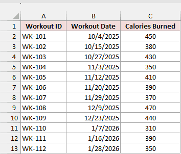
Workout ID is in column A, Workout Date in B, and Calories Burned in C.
Here are the steps to create the monthly average PivotTable:
- Select any cell in the dataset. Go to the Insert tab and click PivotTable.
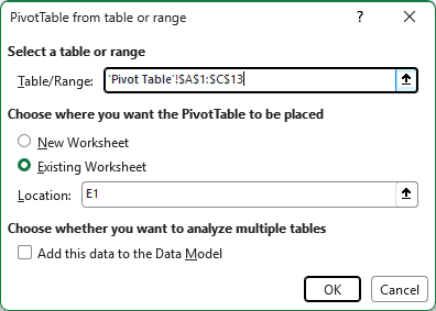
In the PivotTable from table or range dialog, Excel picks up A1:C13. Place the summary beside your workout log using these settings:
- Choose Existing Worksheet.
- Set Location to E1.
- Click OK.
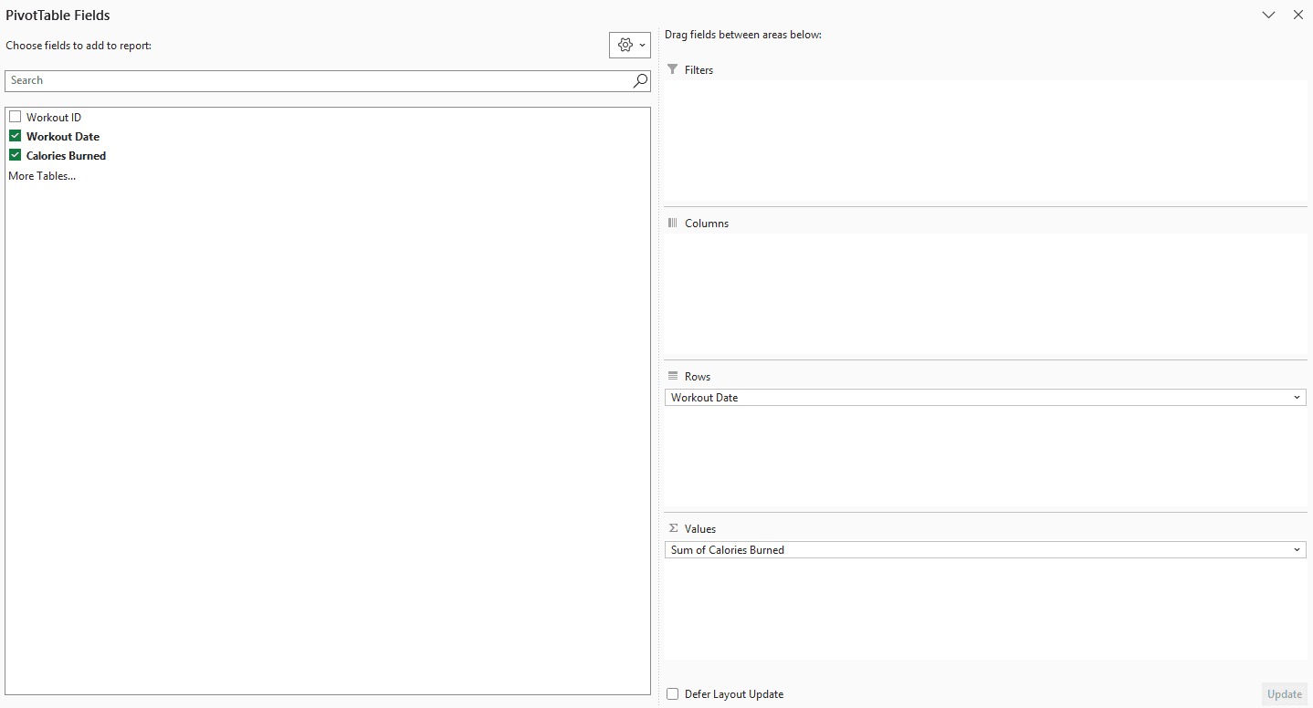
- In the PivotTable Fields pane, drag Workout Date to the Rows area and Calories Burned to the Values area.
You’ll initially see Sum of Calories Burned. Depending on your Excel version and settings, Excel may also group the dates automatically as soon as you add them.
Either way, the next step sets the grouping you want.
- Right-click any date in the PivotTable and choose Group.
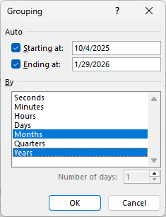
In the Grouping dialog, choose how Excel should collect the dates:
- Select Months and Years.
- Make sure Days and Quarters aren’t selected.
- Click OK.
Include Years to keep January 2025 separate from January 2026. Without it, workouts from the same month in different years would enter one group.
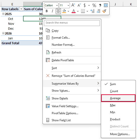
- Right-click any number in the Sum of Calories Burned column. Choose Summarize Values By > Average.
Your PivotTable now shows the average calories burned for each month, grouped beneath its year.
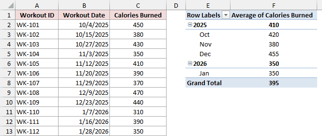
Under Average of Calories Burned, you’ll see October at 420, November at 380, December at 455, and January at 350.
The year rows summarize all workouts within that year. You’ll see 410 for 2025 and 350 for 2026.
The Grand Total, 395, averages all 12 workouts. It doesn’t average the four monthly averages.
Note: A PivotTable doesn’t update automatically when you change the source data. Right-click the PivotTable and choose Refresh to update your summary.
Method #4: Using Power Query
For large logs or recurring imports, you can have Power Query record the steps that turn your workout data into a monthly summary.
It groups your dates and averages the calories without worksheet formulas. When the source changes, you refresh the query to run those steps again.
Below I have a log of 12 workouts, with workout dates and calories burned, and I want the average calories burned for each month.
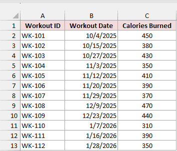
Workout ID is in column A, Workout Date in B, and Calories Burned in C.
Power Query needs your source in an Excel Table. You’ll create that table as you load the log into the editor.
Here are the steps to calculate the monthly averages with Power Query:
- Select any cell in the dataset. On the Data tab, click From Table/Range in the Get & Transform Data group.
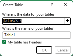
In the Create Table dialog, keep My table has headers checked and click OK. Excel converts your source to a table and opens the Power Query Editor.
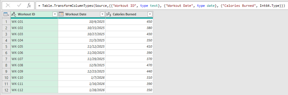
- Click the type icon at the left of the Workout Date header and choose Date. If Excel asks, click Replace current.
Power Query initially reads this column as Date/Time. Left this way, each date carries a 12:00:00 AM time.
The grouped Month column would show times too. Changing the type to Date keeps plain dates.
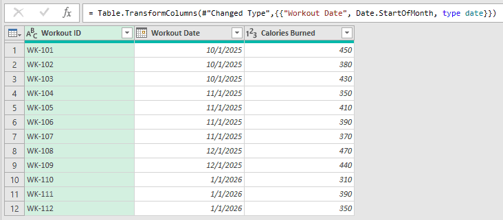
- With Workout Date selected, go to the Transform tab. Click Date > Month > Start of Month.
Each workout date becomes the first day of its month. For example, October 4, 2025 becomes October 1, 2025, giving all October workouts the same date.
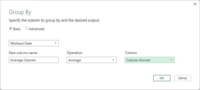
- On the Home tab, click Group By to combine the workouts that now share the same month date.
In the Group By dialog, set up your monthly average calculation:
- Keep Basic selected.
- Group by Workout Date.
- Set New column name to Average Calories.
- Set Operation to Average.
- Set Column to Calories Burned.
- Click OK.
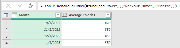
- Double-click the Workout Date header and rename it to Month.
You’ll now have two columns, Month and Average Calories, with one row for each of the four months.
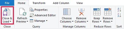
- On the Home tab, click Close & Load.
Excel loads your summary as a new table on a new sheet, occupying A1:B5.
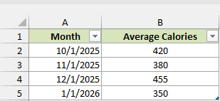
You’ll see 420 beside 10/1/2025, 380 beside 11/1/2025, 455 beside 12/1/2025, and 350 beside 1/1/2026.
The Month column contains the first day of each month. Apply the custom number format mmm yyyy if you’d prefer labels such as Oct 2025.
Power Query records your work in Applied Steps:
- Source
- Changed Type
- Calculated Start of Month
- Grouped Rows
- Renamed Columns
Note: Power Query refreshes manually. After changing the source table, choose Data > Refresh All, or right-click the result table and choose Refresh.
Additional Notes About Calculating Monthly Averages in Excel
Before you use these methods with your own log, check these details:
- Use real Excel dates. Text dates are skipped by AVERAGEIFS and can’t be grouped in a PivotTable. Real dates right-align by default, which gives you a quick check.
- Allow for timestamps. If your dates include times,
"<="&EOMONTH(E2,0)misses entries after midnight on the month’s last day. Use"<"&EOMONTH(E2,0)+1as the second condition instead. - Keep missing values blank. All four methods ignore blank calories cells when averaging. They count zeros, so entering 0 for a missing value pulls your average down.
- Keep the year in your grouping. When your log spans multiple years, grouping by month alone mixes the same month from different years.
Frequently Asked Questions
Here are a few questions that come up when you calculate monthly averages.
How Do I Calculate the Average Monthly Total Instead of the Average Per Month?
Add up each month’s calories first, then average those totals. That answers how many calories you burn in a typical month, rather than per workout.
The monthly totals here are 1260, 1520, 910, and 1050. In Microsoft 365, you can calculate their average with this formula:
=SUM(C2:C13)/COUNTA(UNIQUE(TEXT(B2:B13,"yyyy-mm")))
It returns 1185, dividing the 4740 total calories by the 4 months represented in the log.
Why Does AVERAGEIFS Return #DIV/0! for a Month?
That month has no matching rows, so there’s nothing to average. For example, entering February 1, 2026 in the month list returns #DIV/0! with this log.
If an empty month is expected, wrap the formula in IFERROR to display a blank:
=IFERROR(AVERAGEIFS($C$2:$C$13,$B$2:$B$13,">="&E2,$B$2:$B$13,"<="&EOMONTH(E2,0)),"")
How Do I Average One Month Across Several Years?
To average every January together, match the month number without matching the year. AVERAGEIFS can’t apply MONTH directly to its date range, so use FILTER in Microsoft 365:
=AVERAGE(FILTER(C2:C13,MONTH(B2:B13)=1))
MONTH identifies January with 1. FILTER keeps those workouts, and AVERAGE calculates their average calories. Here, you get 350, because the log contains only January 2026.
Why Doesn’t the Average of My Monthly Averages Match the Overall Average?
Each month gets equal weight when you average monthly averages, even if some months contain fewer workouts.
Here, the four monthly averages average to 401.25, while all 12 workouts average 395.
December has only two workouts, but it counts as a full month in the average of averages. To calculate the overall workout average, use the raw calories:
=AVERAGE(C2:C13)
Conclusion
I’ve shown you four ways to calculate monthly averages, and I’d reach for AVERAGEIFS with EOMONTH as your default.
I hope you found this article helpful.
Other Excel articles you may also like:
