How to Add a Total Row in Excel Table (Step-by-Step)

Excel provides some really great features in the form of Tables. Excel tables provide an organized way of viewing and reporting data in a tabular format.

Besides other advantages, Excel tables provide the option to add a ‘Total row’ to quickly summarize data for each column of your table.

In this tutorial, we will show you how to add a Total Row to your Excel table, after giving a brief run-through on how to convert your dataset into an Excel Table.

Table of Contents

What is an Excel Table?

A lot of people think that the data in an Excel spreadsheet itself is in a table since it is organized into rows and columns. However, your data cannot really be a ‘Table’ until you specify it as one.

An Excel Table is a dynamic set of rows and columns that are pre-formatted and organized, along with various special Table features, like data aggregation, data styling, automatic updates, etc.

The data aggregation comes in the form of a Total Row, which gives you summary calculations for each column, like the sum, average, count, etc. This lets you get an instant overview of your data with minimum effort.

Converting your Dataset into an Excel Table

To view the Total Row, your data has to be first converted to an Excel Table. Let’s say you start with a raw dataset as shown below:

Here are the steps to convert a dataset to an Excel data table:

Click any cell inside your dataset.
From the Home tab, select the ‘Format as Table’ button (found inside the Styles group).
Select the table style that you prefer from the drop-down that appears.
This will display the ‘Format as Table’ dialog box.
Check to see if the range of your dataset displayed under ‘where is the data for your table’ is correct.
You should also see the green marching ants box around the cells that will be included in your table. Correct the range if it does not cover all of your data.
If your data has headers, then make sure the ‘My table has headers’ box is checked.
Click OK.

Note: You can also use the keyboard shortcut CTRL+T instead of steps 2 and 3.

Your dataset should now get converted to an Excel Table. You can tell by the change in the styling of the dataset and the appearance of small arrows in all the cells of the top-most row or header row:

Adding a Total Row to your Excel Table

Once you have your dataset converted to an Excel data table, adding and configuring a Total Row is really easy. There are two ways to do this.

Method 1

Select any cell inside your Excel table.
Select the Design tab of the ribbon (under Table Tools).
In the Table Style Options group, you should see a checkbox next to Total Row.
Check the box to make sure it displays the Total Row at the bottom of your table.

Method 2

Right-click on any cell inside your Excel table.
Select the Table option from the context menu that appears.
Select Totals Row from the sub-menu that appears.

Irrespective of which method you choose, you should now be able to see a Total Row added to the bottom of your table, with the total for the last column displayed.

Once the Total Row gets displayed, you can configure it to display the kind of result you want to see. If you want to see results other than the total, you can click on any cell in the row and you will see a drop-down menu with the available result options.

Using other Aggregating Functions in the Total Row

The ‘Total Row’ gives you the option to display a number of aggregate results, like the average, min, max, Standard deviation, and even the result of a custom function.

For example, say you want to display the Average Selling Price. In that case, here are the steps you need to follow:

Select the cell in the Total Row corresponding to the Selling Price column (cell E7).
You should see a small arrow next to the cell. Click on this arrow.
From the drop-down menu that appears, select the ‘Average’ option.

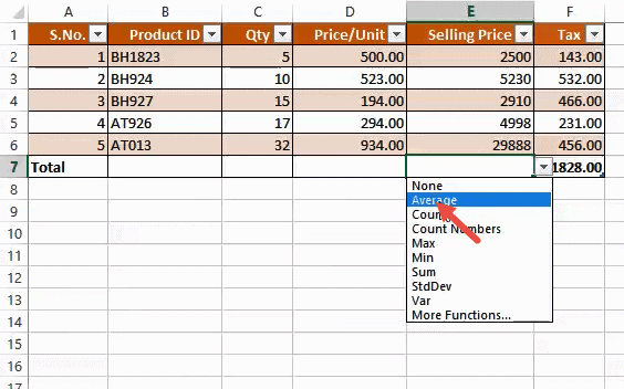
You should now see the average Selling Price displayed in cell E7.

If you click on one of the results displayed, you will notice from the formula bar that most of the aggregate operations in the Total Row use the SUBTOTAL function:

This is because the SUBTOTAL function has the ability to ignore hidden rows. Therefore the calculated aggregates get updated correctly even when the table is filtered.

Note that the aggregating function is completely editable. So, you can easily edit it from the formula bar according to your requirement.

You can also use other functions than the ones displayed in the drop-down. For example, if you want to find a conditional sum of Qty then you can use the SUMIF function as follows:

Select the cell in the Total Row corresponding to the Qty column (cell C7).
You should see a small arrow next to the cell. Click on this arrow.
From the drop-down menu that appears, select the last option, ‘More Functions…’
This will display the ‘Insert Function’ dialog box, from where you can select the function that you want to use.

In conclusion, Excel Tables make it easier for you to work with your data.

One of its useful features is the option to include a Total Row that can help you display results of different types of aggregating functions for a quick overview of your data.

We hope you found this tutorial helpful and easy to follow.

Other Excel tutorials you may also like: