Sequential numbers are an ordered list of consecutive numbers. It can sometimes be needed to have your rows numbered with sequential numbers.
For example, if you have a dataset of different stores in a state, you may want to number the rows and so we have a unique number for each store.
Excel provides multiple ways to enter sequential numbers (also called serial numbers). In this tutorial we will look at 4 such ways:
- Using the Fill handle feature
- Using the ROW function
- Using the SEQUENCE function
- Converting the dataset into a table
Let us take a look at each of these methods one by one to enter serial numbers in Excel.
Using the Fill Handle Feature to Enter Sequential Numbers in Excel
Excel’s Fill Handle feature is smart enough to identify patterns in your data and project the pattern to the rest of the cells in a column.
Say you have the following dataset and you want to enter a sequence of numbers starting from 1 (in the second row) all the way to the last row.
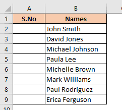
Here’s how you can quickly fill in Column A with a number sequence using the fill handle:
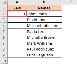
- Enter the number 1 in cell A2.
- Enter the number 2 in cell A3.
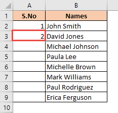
- Select both cells (A2 and A3). You should see a fill handle (small green square) at the bottom right corner of your selection.
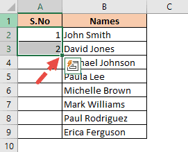
- Drag the fill handle down to the last row of your dataset (or simply double click the fill handle).
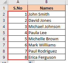
You should automatically get a whole sequence of consecutive numbers, one for each row.
Also read: How to Find the Column Number in Excel
Using the ROW Function to Enter Sequential Numbers in Excel
The above method works great if you simply need to add a sequence of identifiers for each row of your data.
However, your sequencing order will change as soon as you sort the data, or even if you insert/delete a row.
If you need to ensure that the sequencing of the numbers remains the same irrespective of any operations performed on your dataset, then a better option would be to use the ROW function.
The ROW function’s only task is to return the ROW number of the current row.
So if you type the =ROW() in cell A3 or B3 or any cell in row 3, you will get the value 3.
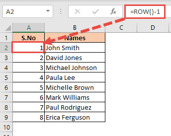
Since we want to start sequencing from the second row onwards (in our example). We can enter the following formula in cell A2:
=ROW()-1
The ROW() function in cell A2 returns the value 2, since it is in the second row.
However, subtracting 1 from the value returned ensures you get one value less for every row number. This means the value in A4 will be 3, and so on.
If, instead of the second row, you needed to start sequencing from the 5th row (say), then your formula would be:
=ROW()-4
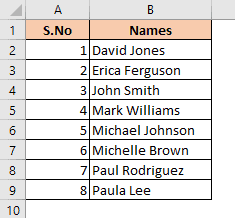
Copy the formula down to the rest of the cells in column A using the fill handle.
You will now be left with a sequence of consecutive numbers, one for each row.
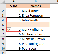
Note that numbering is not going to get messed up even if you sort your dataset or insert/delete rows (in case you insert a new row, just copy and paste the same formula for that new row).
In fact, when you insert a new blank row, the sequencing automatically adjusts itself to ensure that the new row gets its appropriate sequence number.
Also read: How to Square a Number in Excel?
Converting the Dataset into an Excel Table
The above two methods work quite well, but you still need to re-sequence your serial numbers whenever you insert a new row.
If you don’t want to be bothered by this additional hassle, you could simply convert your dataset into a table!
Excel tables are a great tool when working with tabular data as they group the data into a single object, allowing for many additional benefits.
One of the many benefits is that the table automatically inserts formulae or updates them whenever you insert or delete a row in it.
Moreover, even if you add new rows to the end of the table, it automatically expands to include the new rows as part of the table.
This means less hassle for you in updating formulae, and once your table is set up, you never have to bother about updating your serial number column again.
To convert your dataset into an Excel table, follow the steps shown below:
- Select all cells of the dataset.
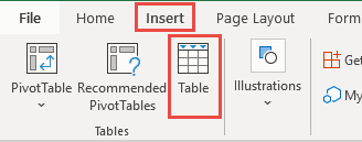
- Navigate to Insert->Table. Alternatively, you could simply press the shortcut CTRL+T from your keyboard.
- This opens the Create Table dialog box. Make sure the range specified under ‘Where is the data for your table’ is correct.
- If your selection included headers, then check the box next to ‘My table has headers’.
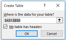
- Click OK.
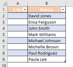
Your selected range of cells should now get converted to an Excel table. You can tell by the change in the formatting of the table:
- Filter arrows appear next to each column header
- The dataset is enclosed in a distinguishable box
- The dataset is styled differently from the rest of the sheet. Rows of the table are styled in alternating colors.
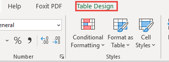
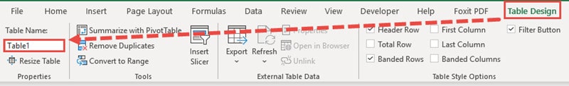
- When you click on any cell in the dataset, the Design (or Table Design) tab appears in the main menu.
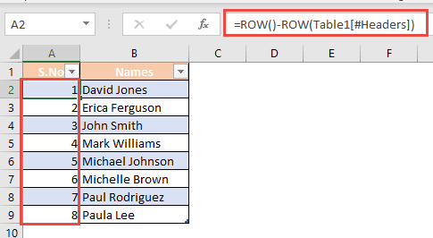
Once your table is ready, you can go ahead and enter the following formula in the first row of your table (cell A2):
=ROW()-ROW(Table1[#Headers])
The above formula simply takes the current row number and subtracts from it the row number of the header row of the current table.
Here, we used Table1 as the name of the Excel table. You can replace this name with the name of your table.
Note: You will find the table name in the Design (or Table Design) tab, in an input box under the label ‘Table Name:’ (when you click on any cell of the table) :
When you press the return key, you should find column A containing a sequence of numbers starting from 1 in cell A2.
This method works irrespective of where your table is located.
Using the SEQUENCE Function to Enter Sequential Numbers in Excel (Only Available in Office 365 and Excel 2021)
Perhaps the easiest way to generate an array of sequential numbers is by using the SEQUENCE function.
The SEQUENCE function is a newly added Excel function. In fact, it is only available in newer versions, like Office 365 and Excel 2021.
This function basically generates sequential numbers in the form of a dynamic array. The syntax for this function is as follows:
SEQUENCE(rows, columns, start, step)
Here,
- rows is the number of rows that you want returned in the array
- columns is the number of columns that you want returned in the array .
- start is the number that you want the sequence to start from. This parameter is optional and by default this value is 1.
- step is the step value by which you want each number of the sequence to increase/decrease. This parameter is optional and by default, this value is 1.
Since we only want a single column of sequential numbers, it is enough to just specify the first parameter in the function. We do not need to add the optional parameters.
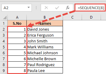
In our example, we want to generate a sequence of 8 consecutive numbers. So we can type the following function in cell A2:
=SEQUENCE(8)
You get an array of 8 sequential numbers displayed in column A as shown:
If you insert a new row into your data, you will notice that the sequence in column A remains put.
However you only have an 8-item array, so your sequence will only last till number 8, even though we now have a new row in our dataset.
Does that mean we have to update the parameter in the SEQUENCE function every time there is an addition or deletion of a row?
Absolutely not.
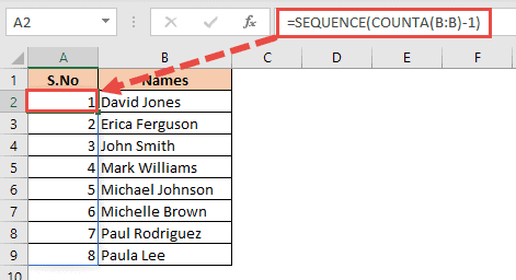
We can use the COUNTA function to keep track of the last row containing data. The following formula should work better:
=SEQUENCE(COUNTA(B:B)-1)
Try removing a row from the dataset.
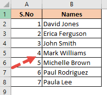
You will notice that the sequence now gets adjusted to display values till number 7 only.
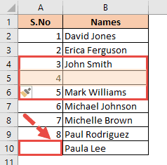
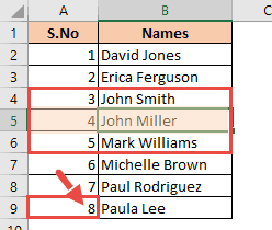
When you introduce a new row into the dataset and enter some data into it, notice the sequencing gets adjusted to accommodate the new row.
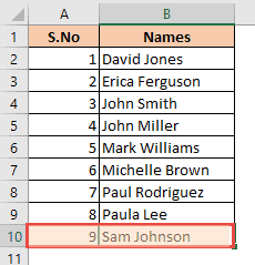
The sequencing also expands as you add newer rows to the end of the dataset.
Note: If your column B contained numeric values (not text), then use the COUNT function instead of COUNTA.
Explanation of the Formula
The COUNTA function simply counts the number of non-null values in a given column.
In our example, the formula: =COUNTA(B:B) will return the value 9, since there are 9 cells in column B (including the header).
But we want to start sequencing from the second row onwards (excluding the header), so we need to subtract 1 from the value returned by the COUNTA function.
Once you get this number, you can then pass it to a SEQUENCE function to get a dynamic array of numbers that change according to the number of rows in column B:
=SEQUENCE(COUNTA(B:B)-1)
When you use this function, you get a sequence of numbers from 1 to 8 (in our case), starting from cell A2.
In this tutorial, we showed you four ways to enter sequential numbers in Excel.
The first method is quite volatile and the sequencing gets easily messed up whenever you alter rows of the dataset.
The second method does away with this issue, but you will still need to re-sequence every time you add, insert or delete a row.
The third method is much more robust, but it involves completely reformatting your dataset into an Excel table.
The fourth method is quite robust as it lets you keep the original formatting of your dataset.
However, the function used in this method (the SEQUENCE function) is only available in newer Excel versions like Office 365 and Excel 2021.
Each method differs in its application and usefulness. You can apply the method that most suits your data.
Other articles you may also like:
Thank you. Your explanation was clear and very helpful.